Concept Deep Dive: Hamiltonian Mechanics
Let's pick up where we left off last time. We now know how to construct a Lagrangian and how to get to equations of motions that way. The Lagrangian though actually needs to be constructed, that is, it's not an actual physical property. One can intuitively show that using something called gauge transformations, which change the Lagrangian by adding a time-integrable term to the end, but keep the equations of motion the same. In physical terms, that wouldn't make a lot of sense if the Lagrangian were more than a means to an end, since any change made to the Lagrangian that way would have to be a change made to either the kinetic or potential energy. If we were to find something that retained the handy attributes of the Lagrangian (or enhanced them), but was a real physical quantity, that would be grand, right? Enter the Hamiltonian. Just in general, the Hamiltonian describes all the energy contained in the system. For mechanics then, we keep the components of the Lagrangian - that is the kinetic and potential terms - and we add them up instead of subtracting one from the other. In a way, if you know how to construct the Lagrangian, you should know how to construct the Hamiltonian, and it's usually how I do it as well. However, there are of course better, more rigorous ways to arrive at the Hamiltonian, which will also help explain their attributes later on.
Legendre Transformation
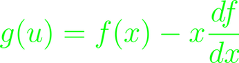
In short, one can arrive at the Hamiltonian by applying the Legendre Transformation to the Lagrangian. However, there are a bunch of assumptions we should probably talk about made before this application is strictly speaking legal, and then most people will use a special form of the Legendre Transformation as well, which exploits some integration attributes of the Lagrangian. First however, I would like to define the Legendre Transformation: For some convex function f, then it's Legendre Transform g is defined by

This immediately raises the question: is the Lagrangian even a convex function? Well, it has to be by construction. We have minimized it in the Integral during construction, so it has to be convex in that area, so even if we have to restrict our Lagrangian to that, that's fine. We wouldn't lose any of its functionality doing that. Now, there's a sense that we do a coordinate transformation here, which isn't necessarily wrong, but also isn't exactly helpful. We're looking for a good transformation that doesn't muck anything up later on.
The Lagrangian doesn't break when put inside a differential, otherwise the second Euler-Lagrange wouldn't make a lot of sense. This is nice to know, since the Legendre Transformation applied to differentials are nice enough to directly give us that transformation (or rather substitution as we will see later). A differential of a function can be generally expanded into a sum of differentials of its dependencies.

A convenient transformation then would be to make the transform dependent on those coefficients in the sum. For some f(x) we can explicate that then to something looking like this
Where of course we want the derivatives to be u, and rewrite the resulting functions as dependent of u. We'll want to apply this to the Lagrangian now, with all its coordinates, and their time derivatives. There's at least more than one dependency in the Lagrangian that we'll treat as independent from one another, which means we'd better know what the Legendre transform of functions with multiple dependencies looks like. The answer is maybe a little anti-climactic, since we have already stated that the dependencies are independent from one another, so we can just treat all but one variables as constant for the purpose of transformation, then iterate over all the dependencies. We have to mess with the signs a bit, or just define the Hamiltonian as the "negative Legendre Transform", to get to where we want to end up:

where we used the generalized momentum to replace the velocities (note, the Hamiltonian retains dependencies of q and t, thus not requiring a Transform for those quantities). Now, this is not as fun to construct as H = T + V, but using the differential of both sides will give us a few very useful relations.

The differentials can be used to do a comparison of coefficients to get

Hamiltonian and Time
Assume some function in phase space, that is taking coordinates, their momenta, and time arguments, and take the total derivative.

The sum and brackets could be packaged into an operator {f, H}, which we'll call "Poisson-Brackets", and this will stand in as the total time derivative if the partial derivative evaluates to zero. This is the case with - for example - the momenta and coordinates themselves. This Poisson-Bracket will play pivotal roles later in Quantum Mechanics where one could generalize this specific attribute for a number of quantities. On the flip-side, let's assume a function whose total derivative with respect to time vanishes. Then, the Poisson-Bracket would be equal to the negative partial derivative with respect to time.
It pays off to inspect some of the attributes the Poisson-Bracket hold. It's - for example - anti-symmetrical, and the Poisson-Bracket of at least one constant is always zero, since there will always be a derivative of a constant in each element of the resulting sum. From the definition, linearity is also easy to prove, since derivatives themselves are linear operations. The product rule for the Poisson-Bracket is also very similar to that of the derivative: {A, BC} = B{A,C} + {A,B}C. Technically, the order isn't very important yet, but it's better to keep it in mind this way, for later applications in Quantum Mechanics. Now, there are proofs out there that require one put a Poisson-Bracket into another one, for which one will require the Jacobi-Identity, which can be proven by computation, but that's not very interesting for our purposes, so I'll just state it here: {A, {B,C}} + {B, {A,C}} + {H, {A,B}} = 0.
A quick look back at those functions whose total time derivative vanishes. Assume we have such a function F, then, along with the asymmetry of the Poisson-Bracket, we get

We call such functions Integrals of Motion. Since the Bracket doesn't need to evaluate to zero, F could still have an explicit time dependence. This separates constants with respect to time from Integrals of Motion, which are non-constant quantities that are conserved within the system.
Hamilton-Jacobi Equation
One could argue, that the Hamilton-Jacobi formulation is a separate formulation to the Hamiltonian, but I tend not to think of it like that, but rather as a transformed Hamiltonian. Given, we arrived at the Hamiltonian using the Legendre Transform, but the Hamilton-Jacobi utilizes something called canonical phase transform, which change the coordinates and momenta to construct another Hamiltonian, meaning it will retain the canonical relations that define the Hamiltonian. Without getting too far into the theory, canonical transformations will result in the following equation after change of coordinates.

The function F is called a "generator", which, depending on the details of the transformation, will yield relations similar to those of the canonical Hamiltonian relations. Because of permutation, there are 4 types of generators for canonical transformations, the second of which is usually convenient. The Hamilton-Jacobi approach will try to find a canonical transformation for which the new coordinates and momenta become constants in time. Then, one can construct a Hamilton-Jacobi differential equation, which will still have the same function as a normal Hamiltonian.

As a side note, the momenta in the Hamiltonian can be written as partial derivatives of F with respect to coordinates. Since the coordinates are now constant in time, there exists an automatic separation between the time-dependent part and the time-independent part, which will become the catalyst for the main approach to solving the differential equation.
Now, I must admit that I don't usually think about this part too much, since I've just rarely found it useful. The Hamilton-Jacobi formulation proves itself useful for Hamiltonians that are integrals of motion, and I can usually make do with the normal Hamiltonian. I don't think I've encountered this much in my studies otherwise either, but in theory, this is the first instance where equating the Hamiltonian and the total energy of the system becomes useful. To me, this approach exists in an odd limbo between too complicated to apply and not useful enough to make the effort for, since where H = E becomes handy next will be in Quantum Mechanics, where the Hamiltonian will become not only our favorite operator, but also our primary Ansatz for solving wave equations. However, in the realm of Quantum Mechanics, the Hamilton-Jacobi Equation gets a challenger that is just a bit too powerful for it to remain useful.
Quantum Mechanics
In the transition from Classical to Quantum Mechanics, there's a couple of things that change in principle, a lot of which is introduced through the inclusion of imaginary space. Equations of motion will transition into wave functions, since all motion will be mapped onto particles with wave properties, and the Poisson-Brackets suddenly change. While getting to the Commutator ([A, B] = AB - BA) can be done from the ground up just as well, these parallels are very firmly grounded in the realm of "because we said so" for now, I think. Later, when delving into Quantum-Field Theory, the reasoning will become clearer, but that is a chapter for another time. The fundamental Poisson-Brackets and the fundamental Commutators change as well, gaining the typical quantum-mechanics factor. The details of all this will be subject for the next go-around.