Concept Deep Dive: Quantum Mechanical Solutions
Having now become familiar with the objects running around in quantum mechanics, we are now ready to look at how to solve the problems whose analogues we've already looked at in the realm of Lagrangian and Hamiltonian mechanics. We are first interested in something that approaches the equations of motion. Although there are equations of motion in quantum mechanics, I would like to do something different first, which I'm rather liable to think of as the analogue to the classical equations of motion.
Some Guy Without His Cat
We understand that applying the Hamiltonian to a wave function gives the Energy as an eigenvalue. This is a sort of eigenvalue equation, which is the Schroedinger Equation in it's simplest form. However, harking back to the Hamilton-Jacobi formulation, we should keep in mind that we can separate the Hamiltonian into a time-dependent and time-independent part. It then is plausible for us to be able to construct a time-independent Schroedinger Equation that looks exactly as described. The time-dependent Schroedinger equation takes into account attribute of the Hamiltonian to function as a time-derivative in the first place. He have to also keep that quantum-mechanical factor in the equation, as well as get sensible expressions for the momentum and position operator in terms of the other respectively in order to remove one degree of uncertainty.

The momentum and its coordinate are nominally independent from one another. We could then separate these two sets of variable into space, called position-space and momentum-space respectively. Since we don't usually have momentum terms in the potential Energy, it's usually sensible to use the position-space representation of the momentum operator.

Knowing some stuff about the wave function often makes the equation relatively easy to solve. As a wave function, we would like the wave function to be finite and continuous. As a probabilistic function, the square of the absolute value should also be equal to one, and since it's meant to be a wave, it should also be oscillating. This is interesting, since, as we'll see later, the potential doesn't actually have to be finite nor continuous.
Potential Walls
Take a potential wall that is infinite at and beyond some place x and zero everywhere else. We can intuitively say that the wave function within that wall has to be equal to zero, and a sine-wave outside of it. At x, the function has to be continuous though, which tells us where it ends, and the energy then characterizes the exponential. Add a second wall to trap the function in, and then the square integral must be equal to one. Technically it's the same for infinite borders, but the evaluation is a little less straight-forward.
For finite walls, the function doesn't need to be zero at the border, but if the potential wall is higher than the energy, this becomes an interesting problem. Obviously the function has to tend toward zero in infinity, but is not zero at the border. The sensible solution here is exponential decay. The full function then is a composite of decays and oscillatory functions.
Harmonic Oscillator Potential
The Hamiltonian of the Harmonic Oscillator gives an expression for the potential.

This gives us the opportunity to do the computation explicitly. First, we would like to know the time-independent solution, so we can add in the time dependency later.

We would like for z to be negligible, and a good way to do that is to find a condition for which y approaches infinity. That lets us apply our usual Ansatz.

This can now be evaluated applying normal differential equations. The solution however will be somewhat long and unsightly, using a series representation of the Hermite-Polynomials. There's an easier way to deal with this specific problem, which utilizes something called Creation and Annihilation Operators. The algebraic approach will reveal a discrete eigenvalue spectrum for the Energy of the harmonic oscillators (as it is with all potentials) of

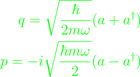
This means that we would probably want to be able to transition a wave function from one Energy eigenvalue to the adjacent ones, with some minimum. Moving the state down an energy-value would be applying an annihilation operator a, and the creation operator would then logically be its adjoint, so that their commutator ends up equal to one. We could then try to associate them with the position and momentum operator in a way, where we can find expressions of the creation and annihilation operators with dependencies of only position and momentum. Those could be used to rewrite the Hamiltonian and solve the problem more or less directly without involving Schroedinger.
Inserted in the Hamiltonian, one arrives at an expression for the Hamiltonian that is equal to that of the Energy, but with the n replaced by the product of creation and annihilation operator. These then define a new operator, the occupation number operator, which is identical to the n in the Energy's index. Moving along the spectrum adds a factor to the state to which the operators are applied:

Hydrogen Atom
Where this occupation number operator makes a lot more intuitive sense is when looking at a hydrogen atom as a quantum system, more specifically at its electrons. With what we know, we can say confidently that the energy spectrum of the hydrogen atom is discrete and since we can always model natural objects with harmonic oscillators, we can even characterize that spectrum to be the same. For electrons, these energy states correlate (somewhat) with the orbitals they exist in. Without going too much into the fine-structure of the atom, the occupation number operator gives the number of particles in the system, hence the name. It's also one of the 4 Quantum Numbers, which are quantities that need to be conserved. In order, there's the occupation number n, which we've already discussed. Then, there's the angular momentum/orbital number l, which gives the magnitude of the orbital angular momentum. It is counted on the orbitals that the particle resides in (s,p,d,f, etc.). The magnetic quantum number m ranges from -l to l and describes the projection of the angular momentum along an axis (usually z). Finally, there is the spin quantum number, which is intrinsic to the particle. The electron for example has the absolute value of one half. Fermions always have half-fractions as spin numbers, bosons have numbers in Z.
All Approximation
So far we've always worked off a large number of assumptions, which generally don't hold true in most physical systems. We usually assume something like a harmonic oscillator, but then if we want to get closer to the actual reality of the problem, we have to do what's called a quantum correction. The basis of this is the perturbation theory, which identifies sources of small errors and tries to counteract them. In a way, quantum physics itself is a perturbation theory to classical physics, which just ignores quantum effects. Implicit here is, that often times we don't need perturbation theory to get a good idea of what we're doing, but at some point, at some time scale that won't be true anymore.
Wanting to correct for "disturbances" in the Hamiltonian is relatively straight-forward in concept. Since the kinetic energy is relatively straight forward, and most crucially almost entirely characterized by the potential and the starting conditions, it is enough to correct for changes in the potential. We thus construct a perturbed Hamiltonian from the "free" Hamiltonian (which we should have solved) and add a small potential correction to the end. Note, that all separations of variables remain intact this way.

This however changes the energy eigenvalues of course. There's a series expansion that helps pulling back changes made to the Hamiltonian and getting an expression of the system in terms of the free Hamiltonian. That one is denoted by an exponated (k), and called the Maclaurin series (in lambda)

One finds, that the new Hamiltonian applied to the power series expansion of the state

is equal the same power series expansion of the energy eigenvalues as a solution. The factors of lambda enables comparisons of coefficients for each of the sums. The zero-th order for example recovers the unperturbed Schroedinger equation. The first order will have two different kets (order 0 for the free Hamiltonian, order 1 for the potential correction), which in itself can be placed under comparison of coefficients. Since the energy terms are scalar (because physics cries otherwise), one could eliminate the vectors on the energy-side, which would create a concrete value for the first order energy shift.

We are operating under the assumption that under the bra-ket with nothing in between evaluates to one. For normalization, the zero-th Maclaurin of the n-state also is one. From there one can conclude through computation that mixed Maclaurin bra-kets are zero. From here, the corrections can go as high as we want, but we'll always ignore some high-order term of lambda, which operates under assumption that lambda is very small. With this, we only need to know basic things about the energy spectrum (not their exact value), such as their degeneracy, i.e. whether they have a multiplicity larger than one in the system to complete the computation up to whichever order we want, though the algebraic cost will rise rather rapidly as we go on.