Functional Analysis

Lᴾ-Spaces and Banach Spaces

New year, new book! That last one was hard to digest as well, and I'm kinda glad to be done with it (more or less). It was a very tight two months, and trying to understand such dense topics put me right up against the limitations of my schedule, but I managed to get through it mostly without incidents. I think I'll check out something different for the next few weeks.

I've once tried studying functional analysis, but with terminal topology brain, most professors won't agree with your proofs anymore, it seems, but I think a lot of the topics are still interesting, even though analysis has lost some of its charm to me since that experience. I'm using the book on Functional Analysis by Elias M. Stein and Rami Shakarchi. I'll assume that the basic concept of an Lᴾ-space and Banach space is familiar to the readers. The definition is quite easy to look up and understand, but writing it down digitally would involve a lot of LaTeX, which I'm choosing to avoid where possible.

Let's remind ourselves of two fundamental inequalities in analysis. For some dual exponents p, q the Holder inequality is:

The Minkowski inequality is:

These can be used for getting proving that all manner of spaces are complete (vector) spaces.

Banach spaces are complete normed vector spaces. Spaces are considered complete, if all Cauchy sequences within it, converge inside it. A linear functional is a linear map l from some Banach space B to ℝ, so that l(af + bg) = al(f) + bl(g) for all a, b ∈ ℝ and f, g ∈ B. They inherit the continuity and boundedness properties for all regular functions. Linear functionals on Banach spaces are continuous iff they are bounded. Given the norm

the B, equipped with this norm is the dual space B*. For Lᴾ spaces, their duals use the dual exponent q instead of p. These are unique, since they're fixed on the constant 1. For conjugate exponents p, q, one can also define

for some integrable g. A linear subspace V₀ with a linear functional l₀ so that l₀(v) ≤ p(v) contains an extension l on V so that l(v) ≤ p(v). This is the Hahn-Banach theorem. It implies that elements f₀ of a Banach spaces that have norms ||f₀|| = M has a continuous linear functional l on B with l(f₀) = M, and ||l|| = 1. Since linear transformations are dual, pairs of Banach spaces B, C with a map T between them, so that T(af + bg) = aT(f) + bT(g), and it's bound by ||T(f)|| ≤ M||f||. Keep in mind that T(f) lives on C and f lives on B, and to take the correct norms. If S is a dense linear subspace of B and T₀ a linear transformation from S to C, satisfying the previous condition, then T₀ has a unique extension T to all of B with the same property. There is also a linear transformation T* in between the dual spaces C* to B* so that T*(l₂)(f₁) = l₂(T(f₁)).

There exists an extended, non-negative function m, so that for two disjoint subsets E, F of ℝ, m(E ∪ F) = m(E) + m(F). m(E) = n(E) if E is measurable and n is its Lebesgue measure. m(E + h) = m(E) for all E and real numbers h. Such functions can also be found on all subsets of ℝ/ℤ. For Lebesgue integrals, there exists a linear functional f (onto I(f)) on all bounded functions on ℝ/ℤ, so that I(f) ≥ 0, if f(x) ≥ 0, I(f) is the integral of f(x) from 0 to 1, if f is measurable, and I(f(x-h)) = I(f) for all real numbers h.

The dual to the space of continuous real-valued functions on X: C(X) can be probably best described by their elements. for all l ∈ C(X)*:

For this, the properties of continuous functions will be useful. Separation is the property that for A, B two disjoint closed subsets of X, there is a continuous function f with f = 1 on A, f = 0 on B, and 0 < f < 1 in their complements. The partition of unity is the property that for compact sets K covered by finitely many open sets, there are continuous functions for each of these open sets, that exist between 0 and 1, so that their sum equals 1 for all x in K. In general, their sum should also exist between 0 and 1.

In the case of positive linear functionals, meaning functionals that are positive, when their argument is a positive function, these are bounded automatically, and ||l|| = l(1). On a compact metric space, there is a unique finite and positive Borel measure μ:

If l is instead only bounded, then it can be decomposed into positive linear functionals l⁺, l⁻ with l = l⁺ - l⁻ with ||l|| = l⁺(1) + l⁻(1). If C(X) is the Banach-space of continuous real-valued functions, then there is a unique finite signed Borel measure on X:

C(X)* will also be isometric to M(X). A metric space X and positive linear functional l on Cₜ(X). Let l be normalized to l(1) = 1 and all ϵ > 0, there is a compact set Kϵ ⊂ X with

Lᴾ-Spaces in Harmonic Analysis

A lot of this chapter circles back to this statement: A linear mapping from sums of L-spaces T, so that

A holomorphic function f in the strip S = {z ∈ ℂ: 0 < Re(z) < 1}, which is also continuous and bounded on ∂S, implies

This is the "three-lines theorem", describing that the size of f on the line Re(z) = t is controlled by its size on its boundaries at Re(z) = 0 and Re(z) = 1. Assume that T is defined on simple functions of X, and maps to an integrable set with finite measure Y. For the mapping as described at top to exist, one can define the "Riesz diagram" of T. It consists of all points in {(x, y): 0 ≤ x ≤ 1, 0 ≤ y ≤ 1}. This is a convex set. For dual exponents p, q and 1 ≤ p ≤ 2:

and the Fourier transform T has a unique extension to a bounded map between the L-spaces, as described up top. Applying this formalism to a construction that extends the unit circle by ℝ and the unit disc to the upper half plane ℝ²₊ moves the theory onto Hilbert spaces. For this, we note the Plancherel's theorem and Hilbert transform as:

H is unitary on L², and H² = -I. The Hilbert transform can be written as a singular integral, from which emerge definitions of the Poisson kernel and its conjugate

This is the L² theorem. Expanding this to the general case of the Lᴾ-theorem, leaves us with the inequality

where A is bound and independent f, and where the Hilbert transform has a unique extension to Lᴾ in its entirety under the same bound condition. The maximal function of any function f on an Lᴾ space is defined as

where B is an arbitrary ball containing both x and m, with a radius greater than dy. It can also inserted into the Lᴾ inequality. There is a weaker inquality for bound A, so that

A distribution function λ can be defined on non-negative measurable functions F for positive a, so that λ(a) = m({x : F(x) > a}). It has an integral version.

which will also be true if one of the sides turns out to be infinite. This expression can be shown using the Tchebychev Inequality.

A space that is very similar to real Lᴾ-spaces are real Hardy spaces. The Lᴾ inequalities occasionally break down at p = 1 for the Hardy spaces were first defined. Hᴾ for the upper half-plane consists of holomorphic functions F on the upper half-plane with

with the p-th root of the left side as the norm of F. For F ∈ Hᴾ, the limit of F(x + iy) for y approaching 0 exists in the Lᴾ norm. H¹ᵣ(ℝ) is the space of real-valued functions so that 2F₀ = f + iH(f) with F ∈ H¹. This definition can be extended for higher-dimensional real spaces. Bounded measurable functions a on M = ℝᵈ is considered an "atom" to a Ball B in M, if a is supported in B, so that |a(x)| ≤ 1/m(B) for all x and ∫a(x)dx = 0. The Hardy space consists of all L¹ functions can be written as an infinite sum of scaled atoms, where the sum of all absolute coefficients is finite. The norm of the Hardy space is complete, so it's a Banach space. If f ∈ Lᴾ(ℝᵈ), p > 1 has bounded support, then it is part of the Hardy space iff its integral over ℝᵈ vanishes. A non-trivial open set O in ℝᵈ, a collection of dyadic cubes with disjoint interiors exists, so that O is the unification of these cubes, and diam(Qᵢ) ≤ d(Qᵢ, Oⁿ) ≤ 4 diam(Qᵢ). The atomic decomposition of the Hardy space can then be articulated more generally by defining a p-atom (p > 1) associated to a ball B in which it's supported and

Any p-atom is an element of the Hardy space, and there exists a bound constant cₚ so that ||a|| ≤ cₚ. Elements of the Hardy space can be Hilbert-transformed into elements of L¹. This transformation converges in the L¹ norm. For a limit, a maximal function can be defined given another function, which is bounded and has compact support:

For a suitable constant c, |f(x)| ≤ M(f)(x) ≤ cf*(x) for all function in L¹. If Φ is a C¹ function with compact support and the corresponding maximal function M, M(f) is in L¹ if it's in H¹ᵣ.

For the case of infinite p, a different space can serve as a replacement to the Lᴾ space. This is the "Bounded Mean Oscillation" (BMO) - the dual space of the Hardy space - with elements f, so that

This is taken as the BMO-norm. Null elements in BMO are constant functions. The space of real-valued BMO functions forms a lattice. Linear functionals l of the Hardy space can be written as

This integral doesn't always converge, so l requires a unique extension to the Hardy space, so that

Distributions

A generalized function or "distribution" F doesn't assign values at "most" points, but is assigned averages taken with respect to smooth functions. With test functions φ: F(φ) = ∫f(x)φ(x) dx. There are two classes of distributions, a broader one defined on any real open set, and those tempered at infinity. "Test functions" for a class of distributions are functions that are infinitely differentiable at 0 in compact support of the set. Distributions are complex-valued linear and continuous functionals. For legibility, distributions are usually noted down in capitals, and functions in lowercase. Examples of common distributions include the "Dirac-Delta function", somewhat of a misnomer. The derivative for distributions can be applied without any real difficulties, but it's technically a generalization of the operator. The usual operators, such as translations, Fourier transformations and scaling operators, can be easily applied to distributions. One of the most relevant ones is the "convolution"

The identity from both sides of the convolution is the Dirac-Delta distribution. Appropriate inputs for the convolutions are infinitely differentiable, and the results of a convolution is as well. The support of a continuous function f is the closure of the set, where f(x) ≠ 0. It's the complement of the largest open set, on which f(x) = 0. The latter definition can be applied to distributions much better than the former one. Formally, it's the correct one. The support of a convolution is the (outer) sum of the supports of the inputs. There is a space of test functions on ℝᵈ, called the Schwarz function, noted as S. Tempered distributions are continuous, linear functionals on S. The vector space of tempered distributions is S*. For a tempered distribution F, there is a positive integer N, and a positive constant c with |F(φ)| ≤ c||φ|| for all φ ∈ S. The Fourier-transform of distributions of compact support is a slowly increasing, infinitely differentiable function. Distributions are allowed to have isolated points as supports, whereas functions require continuity for support. Assume the distribution F is supported at the origin, then it can be written as an infinite sum

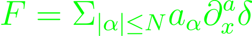
If it's tempered and F(xⁿ) = 0 for all |n| ≤ N, then it's the flat zero-distribution. The function 1/x is not a distribution, because it's non-integrable at x = 0. The "principal value" is somewhat of a replacement for this function in the realm of distributions.

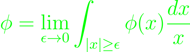
The principal value functions as the 1/x distribution for all intents and purposes. Note that it evaluates to 0 near x = 0. We note it as "pv(1/x)". It's a homogeneous distribution. A distribution is homogeneous of degree d, if Fₙ = nᵈF for all positive n, where Fₙ(φ) = F(φⁿ). Tempered distributions with homogeneous degree g in ℝᵈ has a Fourier transform with degree: - d - g. Assuming -d < g < 0, then

To generalize the Hilbert transform with corresponding Lᴾ-theory, introduce (first) the convolution operator T(f) = f*K, where K is a regular distribution. For K exists an infinitely differentiable function k, which coincides with K away from the origin. Then,

k has a "cancellation condition": C(n)-normalized bump function φ is supported in the unit ball, and

Kernels K of this type are "Calderon-Zygmund distributions". The operator T extends to a bounded operator on Lᴾ(ℝᵈ) for finite p > 1.

T then has a unique extension with this bound condition to all of Lᴾ.

Baire Category Theorem

Sets in metric spaces can be can be separated into two categories. It's considered to be part of the first category, if it's a countable union of subsets that whose interiors of its closure is empty. Such subsets are considered "nowhere dense". Those sets, for which this is not true, are automatically part of the second category. If a set in the second category is the complement of a set in the first, it's considered "generic". Every complete metric space is then of the second category. In complete metric spaces, generic sets are always dense. A sequence {fₙ} of continuous complex functions on a complete metric space X, so that the limit of the sequence is defined everywhere. The sets of points where f is continuous is generic. f is only discontinuous on a set of points within the first category - i.e. at "most" points. Given an open ball B in X,

On C([0,1]), the set of functions that are nowhere differentiable is generic. On a Banach-space B, L is a collection of continuous linear functionals. If sup|l(f)| < ∞ ∀ f ∈ B, then sup ||l|| < ∞. This is also true, if f is in a set of the second category. If B is limited to ±π, there exists a continuous function with a defined Fourier series on B, but which diverges within it as well. The set of such functions is generic as well.

Let X, Y be Banach spaces with norms, and T: X → Y a mapping. T is continuous iff {x ∈ X: T(x) ∈ O) is open in X for open O in Y. If T has a continuous inverse, T is considered an "open mapping". This happens to coincide with surjectivity of T. A bijective, continuous linear transformation implies a continuous inverse, so that constants c, C > 0 exist with

A mapping T given by T(f) = {f(n)} is linear, continuous, injective, but not surjective. There are complex sequences, that vanish at infinity, but aren't Fourier coefficients of L¹-functions. For two Banach-spaces, a linear map can be defined as a graph, as a subset of X ⨉ Y:

T is closed, if its graph is a closed subset in X ⨉ Y. Continuity can be rephrased as a closed linear map. A finite measure space (X, F, μ). Then, a closed subspace E of Lᴾ(X, μ) with a finite p ≤ 1, which is contained in L(X, μ), then E is finite-dimensional. From this follows that there is an A > 0:

A "Besicovitch set" is a compact set with two-dimensional Lebesgue measure zero, containing unit-line segments in all directions. It can be constructed as a union of finitely many rotations of a set, which was given as a union of line segments joining points between Cantor-like sets on the lines y = 0, and y = 1. On the compact subsets of the square Q = [-1/2, 1/2] ⨉ [0, 1] consisting of a union of line segments joining points from N = {-1/2 ≤ x ≤ 1/2, y = 0} to M = {-1/2 ≤ x ≤ 1/2, y = 1}, to all directions. Name K the set of closed subsets of Q, so that each subset is a union of line segments l joining a point of N to one of M, and that every angle between ± π/4 has a line segment l. K is a closed subset of the metric space, so adding the Hausdorff distance to K, makes it a complete metric space. The collection of sets in K of 2-D Lebesgue measure zero is generic. Importantly, it's non-empty, and as such, dense. This follows from the observation that sets in K with horizontal slices with "small" Lebesgue measures are generic. For each fixed point, and infinitesimal distance, the collection of sets within the infinitesimal distance around said point is open and dense in K.

Semisimple Lie Groups SU(N) (N ≥ 2)

This is a special case of non-Abelian gauge groups, which is especially relevant to characterize the fundamental forces for at least the standard model, and must set the motivation for alterations to it. SU(N) in its fundamental representation consists of a product of unitary N ⨉ N matrices with positive determinants, which are themselves associated with linear, special unitary transformations of a complex vector space. From previous entries, we should know both that SU(N) is a continuous Lie group, and the definitions of Lie groups. For the intuition of the following, Lie groups should be thought of as differentiable manifolds. Elements of a Lie group may be expanded about the unit element as

with traceless and Hermitian generators t, structure constants f, and some distance parameter ξ from unity. This distance may be represented by the exponential of iξt, meaning an infinite series of infinitesimal transformations. The generators span a vector space, with dimension N² - 1 for SU(N). In the following, we note the Lie algebra of a Lie group G as g.

SU(N) is semisimple insofar that its Lie algebra su(N) is a direct sum of simple Lie algebras. See the course on fundamentals of algebra for a more rigorous definition of simple algebras. Within physics, it's convenient to map the group action of SU(N) onto a space determined by the spin properties of a particle, using a representation of dimension 2J + 1 where J is the total spin (half integer, starting with 0). The Weyl theorem implies that this representation is completely reducible. For irreducible representations r of SU(N), their generators can be normalized down to a coefficient that is consistent with the structure constants.

In Yang-Mills theory, the standard representation of a Lie group is spanned by the generators, i.e. its own Lie algebra, so that the adjoint representation are given directly by the structure constants with maximal dimension.

with a representation-dependent constant C. For SU(2), the generators can be normalized into the 2D fundamental representations built through the 2-Pauli-matrices.

For later use, define the center of SU(N)

Bernoulli Trials

There is a way to derive the central limit theorem from the idea of mutually independent random functions, so called "Rademacher functions", which in turn can be studied using Bernoulli trials as proxy. The easiest Bernoulli trial is of course the coin flip, the basics of which I'm assuming is familiar to the reader. Key concepts include the stochastic definition for events and probability spaces, the binomial coefficients and Stirling's formula. Things get interesting for the case of infinite iterations.

First, the probability space is trivially the infinite product of ℤ₂. For simplicity's sake, we note it as X in this entry. X inherits the natural product measure from its components. The cylinder sets E in X with n-long events of a subset of ℤ₂ⁿ have finite unions and intersections and complements. They form an algebra on X. The function m(E) = mₙ(E') as the measure, extends to a measure of the σ-algebra of sets generated by the cylinder sets. m(X) = 1. The measurable sets / events and the measure m of the σ-algebra with m(X) = 1 forms a pair (X, m). X becomes the probability space, and m the probability measure. Extending the product measure to a finite set of functions r can be defined to set a correspondence between X and [0, 1] with the measure m through the following map

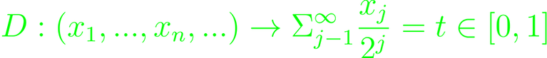
Removing Z₁, Z₂ makes D a bijection, for Z₁ contains all points with all 0/1 entries after a finite number of places, and Z₂ contains all dyadic rationals. Let E be the cylinder set of X with all coordinates that are of a given finite set of 0s and 1s. D then maps E onto the dyadic interval

To obtain the Rademacher functions, write the functions r as functions of t in [0, 1] and extend them to r by making it periodic of period 1. Given some (X, m), a sequence of real-valued measurable functions f on X are mutually independent, if for any sequence of Borel sets in ℝ

(X, m) can also be written as a product of probability spaces.

For any positive integer, since {r(t)} forms an orthonormal system on L²([0, 1]),

A sequence of functions {fₙ} converges to f in probability, if

The central limit theorem can thus be defined using the distribution measures. For real-valued functions f on a probability space (X, m), the distribution measure is the unique Borel measure on the rational number space, so that

A measure that arises naturally in many such descriptions is the Gaussian distribution. Applying the central limit theorem in the context of coin flips, sees a convergence toward the normal distribution.

Randomness in series can lead to convergence where an ordered series would not otherwise converge. This is true for the geometric series with a random sign preceding the elements, for example. However, for almost all t in [0, 1]

The inverse is true, if the series diverges. A series of Rademacher functions that Lipschitz-converges with its length for almost all t, also converges for exponents larger than one half of its length.For a subset E of [0, 1] and m(E) > 0, there is a coefficient c > 0 and some N > 0, so that

The mutual independence of the Rademacher functions give a version of orthogonality. For finite F

From this, series with some squared coefficients that converge, define a Fourier transform with its coefficient for almost all t in [0, 1]. The inverse is true, if the series diverges.

Sums of Independent Random Variables

For large numbers in statistical processes, one should be familiar with the law of large numbers, and perhaps a little less familiar with the ergodic theorem. Both can be shown with the theorems from the previous week. Functions are ''identically distributed'', if the distribution measures are independent of the index used in the sequence. Their measures are then identical for all n in all Borel sets. If a sequence is identically distributed and if the first function in the sequence has a mean, then all other functions have the same mean. It follows, that

Sequences of functions have the same joint distribution, if for all real dimensional spaces, their measures are the same, regardless of Borel sets. For such sets with the same joint distributions, the sequences of continuous functions derived from these sets also have a joint distribution. They also share their mean almost everywhere. With an integrable function f and sub-algebra A of the space of measurable sets M has a unique function F, so that F is A-measurable, and the integrals of f and F over their respective sub-algebras are equal. This can be used to make a guess about the integrals of complicated functions. A sequence of mutually independent, integrable functions with mean zero implies the existence of an increasing family of sub-algebras, defining the martingale sequence

Square integrable independent functions with mean zero and a standard L²-variance, which, if summed up in a series, converge, creates a converging martingale function. If the infinite martingale function is integrable, and generally

and if sₙ converges in L¹, it does so everywhere to the same limit. A sequence of sub-algebras of M define a "tail algebra"

If the algebras are also mutually independent, then all elements of the tail algebra have measures of either 0 or 1. The same can then be transferred to mutually indpendent functions. Using identically distributed and square integrable functions with the same mean and variance leads to

To prove this, it might be handy to know that measures are continuous, if each point has measure zero.

If the functions are not real-valued, but instead ℝᵈ-valued, then it can be written as a vector of d real-valued functions. The distribution measure then becomes the non-negative Borel measure

The definition for integrability can be extended to different, usually stronger forms of integrability. Square integrable d-dimensional functions define a covariant matrix of f.

It's symmetric and non-negative with a unique square root. The sequence of ℝᵈ-valued functions are mutually independent, if their algebras are all mutually independent. This independence carries with all constant vectors, obviously. The characteristic function of an ℝᵈ-valued function is its d-dimensional Fourier transform. A sequence of mutually independent, identically distributed and square integrable ℝᵈ-valued functions with mean zero, an invertible covariant matrix, will have a measures on ℝᵈ that converge weakly toward

This can be modeled onto a random walk process

Brownian Motion

Brownian motion can be modeled using the random walk sequence any probability space with measure m. Joining the points this sequence generates a path that can be normalized to a set time interval. This is a stochastic process. To get to the proper formulation, first one should identify the probability space for Brownian motion (Ω, P), where P is the probability measure, and ω is a typical point in Ω (so a real-valued d-dimensional vector). For zero time steps, the Brownian motion process is assumed to be zero almost everywhere. The incremental steps are independent of one another, and they have a pairwise Gaussian covariance with mean zero. Except for quirks in the measure, the resulting path should be continuous. Each step is also normally distributed with mean zero. There is a natural choice for the canonical description, depending on the probability space Ω. Due to the continuity of the path, the resulting inclusion leads to a choice of probability measure P with a corresponding measure W on P³. This is the "Wiener measure". It needs to satisfy the properties of Brownian motion, in a way, characterizing the concept. It is unique for each P. The probability measure on P is induced via the metric and converges weakly to the Wiener measure.

For paths in P, introduce a metric

P here is separable and complete with respect to said metric d. The Borel sets B of P is the same as the σ-algebra generated by the open balls in P. The proof is taken from the cylindrical set of Borel sets. Define a section of μ to be the measure on the metric space. If two sequences are identical for the same sets of times, then their measures are identical. Sequences of measures may converge weakly to some probability measure. If it exists on a metric space, then the sequence is tight, if its measure assigns proper (less than 1) probabilities to all compact sets of the metric space

If the sequence is tight, then it has a weakly converging subsequence. Any tight sequence of weakly converging subsequences, itself converges weakly. A closed set in P is compact, if there is a positive bounded function f for all positive T, so that

The measures on P converges weakly toward the Wiener measure. Given a Wiener measure on P,

Markov Property and Dirichlet Problem

Take a bounded, open, d-dimensional set and a continuous function f on the boundary. Find a function u, that is continous on the enclosure and is harmonic in R, that converges toward f on the boundary. Brownian motion factors into the problem when fixing a point in R as a start of a Brownian motion process. For all subsequent motions, the resulting induced measure on the boundary is given by

ω → τ(ω) maps the "stopping time". The martingale sequence {sₙ} associated to the increasing sequence of the σ-algebras on the probability space (X, m). The stopping time is an integer-valued function.

Brownian motion is essentially a continuous version of a martingale series. For all (sensible) times t, the σ-algebra generated by all the functions Bₛ, 0 ≤ s ≤ t. Then, sequence {Bₙ} is a martinglae relative to {Aₙ}, and for almost all ω, the path Bₜ(ω) is continuous in t. The maximal inequality immediately leads to the familiar Brownian motion inequality. Two different, well defined "natural stopping times" arise, one is the exit time, and one is the strict exit time.

The stopping time σ can also define a collection A with sets a so that a ∩ {σ(ω) ≤ t} ∈ A for all non-negative t. Suppose a Brownian motion B and stopping time σ, then define another Brownian motion, which is independent of its underlying σ-algebra.

Successive Brownian motion processes are then entirely independent of one another's starting positions. This is the Markov Property. Other forms of this property are embedded in the Borel functions. For a Borel function on the space of all paths:

The Markov property can also be applied to the Dirichlet problem directly. Once again, with two stopping times, defined the stopped process.

For u defined as at the beginning of the section, we can remember that u is harmonic in R, and u(x) → f(y), as x → y. For a regular point y on the boundary of R,

This fixes the upper and lower bounds of the function, since y is regular. s, ϵ > 0 can be used for limiting the function values.

Hartog's Theorem

The following will work extensively with holomorphic functions on complex spaces. While these objects are pretty much omnipresent, but some other definitions might be in order. A polydisc is a product defined on n-dimensional complex coordinates and an n-dimensional vector r.

Holomorphic complex functions gain satisfy the Cauchy-Riemann equations, meaning that they also have a Cauchy integral representation. In fact, these properties are equivalent for continuous functions on open sets. A pair of holomorphic functions in a region, that agree in a neighborhood of some point within said region will agree throughout the entire region. If F is holomorphic on a region O containing the union of K₁ = {(z₁, z₂): |z₁| ≤ a, |z₂| = b₁}, K₂ = {(z₁, z₂): |z₁| = a, b₂ ≤ |z₂| ≤ b₁}, then it extends analytically to an open set containing the product set {(z₁, z₂): |z₁| ≤ a, b₂ ≤ |z₂| ≤ b₁}. This also means that if F is holomorphic in Ω = {z \in ℂⁿ, ρ < |z| < 1} for fixed ρ between 0 and 1, it can be analytically continued into the a complex n-Ball with radius 1. For n > 1, the function can't have an isolated singularity or isolated zero, and holomorphic functions inside the unit ball can't necessarily be extended outside it. The generalized study of these analytical continuations requires some use of inhomogeneous Cauchy-Riemann equations.

The case of n = 1 is easy and immediately solvable, the complexity of the solution scales with dimension. If f is continuous with compact support on ℂ, then the solution is given by this one-dimensional solution, and satisfies the one-dimensional Cauchy-Riemann equations. If f is in the class Cᵏ, k > 0, then its solution satisfies the one-dimensional Cauchy-Riemann equation as well. Functions in C¹ with compact support are automatically solutions of the 1D Cauchy-Riemann equation. If n > 1, then f must be functions of class Cᵏ of compact support, satisfying the CR consistency condition

and a function u exists satisfying the inhomogeneous CR equations. This yields a general form of Hartog's principle for ℂⁿ, n ≥ 2, and K a compact subset of Ω with connected Ω - K. Any function analytic in Ω - K has an analytic continuation in Ω. A defining function in ℝᵈ is a real valued function with

if ρ is of class Cᵏ, and |∇ρ(x)| > 0, then Ω is considered to be of class Cᵏ as well. The boundary then is a hypersurface of class Cᵏ. A local hypersurface M of class Cᵏ is given by a real Cᵏ function on a ball in ℝᵈ, so that the points in the ball evaluate said function to zero.

The Levi Form

In ℝᵈ any boundary point, the near region can be put in very simple canonical form by choosing appropriate coordinates, so that the region is represented through functions and mapped onto the half-space with a vanishing hyperplane for a boundary. To transfer this intuition to complex holomorphic functions, the new coordinates need to be expressed through holomorphic functions. These are referred to as "holomorphic coordinates". Near points on the boundary, holomorphic coordinates {z} can be introduced, so that they are centered at that point, and the area is

This is facilitated directly by a Hermitian matrix which, when diagonalized becomes the sum in the above formula. When in the summed form, it's referred to as the "Levi Form" of Ω at the boundary point. The transformed unit vectors are tangent to the area boundary, so with ρ(z) = φ(z', xₙ) - yₙ, it can be written in a quadratic form.

A biholonomic map ω near the origin creates a holomorphic coordinate system, so the differential maps tangent vectors to tangent vectors of one lesser order. A boundary point of Ω is "pseudo-convex" if the Levi-form is non-negative, and "strongly pseudo-convex" if it's strictly positive. If this is true for the entire boundary, then Ω inherits the property. For n > 1, the Levi form can experience a "local" maximum principle in ℂⁿ. For an open ball around Ω with a boundary in ℂ² and an open ball B centered at a boundary point z⁰. All points in the intersection between ball and boundary have at least one strictly positive eigenvalue of the Levi-form. A smaller ball B' exists in B, centered in z⁰, so that holomorphic functions F on Ω ∩ B, continuous on its completion have

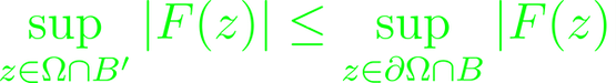
This is true in the more general case for a local hypersurface instead of the boundary.

The classical Weierstrass approximation theorem may be restated so that given a continuous function on a compact segment on the real axis in complex space, f can be uniformly approximated by polynomials in coordinates of z = x + iy. A complex n-hypersurface M with n = 2 or larger, will haven open ball B', B centered along M with the closure of B' in B, so that if a continuous function F in the intersection of M and B satisfies the tangential Cauchy-Riemann equations in the weak sense, then F can be uniformly approximated on the intersection of M and the closure of B' through polynomials in {z}. This is true for all strictly positive integers n. If n = 1, there are no tangential Cauchy-Riemann equations, so it's trivially valid. For n > 1, there are no requirements for the Levi-form of M. If the Levi-form has at least one strictly positive eigenvalue for all points on M, then for all centers of balls B' in M with continuous functions F satisfying the tangential Cauchy-Riemann equations in the weak sense, then there are holomorphic functions G in the lower half-sphere of B' continuous on the closure of the lower half-sphere of B', so that G and F coincide on the intersection of M and B'.

Oscillatory Integrals

Oscillatory integrals I(λ) generally have the form

and become interesting at large (and real) λ. Usually it's assumed that the phase and amplitude are real-valued. The principle of stationary phase says that while the gradient of the phase is non-vanishing, the integral rapidly decreases in λ and the dependency becomes negligible, and the main contribution of I(λ) is reduced to the points, where the gradient of the phase vanishes. For |∇Φ(x)| ≥ c > 0 for all x in the support of φ, then for every N ≥ 0,

For N = 1, c can be assumed to be 3. Check first the case for a static phase for some point x, and a non-degenerate critical point. For a phase of x²

The curvature form or second fundamental form of a surface M is

restricted to tangent vectors to M. It is independent of normalized defining functions.

where the eigenvalues λ are the "principal curvatures" of M at a critical point, and their product forms the total curvature / Gauss curvature of M. Next check the induced Lebesgue measure dσ on M. For any continuous function on M with compact support,

A measure dμ is a surface-carried measure on M with smooth density, if dμ = φdσ, and φ is a C[∞] function of compact support.

For hypersurfaces M with surface-carried measures dμ, define a map A

A is the averaging operator. In Riesz diagrams, A forms a closed triangle in the (1/p, 1/q) plane with (0,0) (1,1), (d/(d+1), 1/(d+1)). For a hypersurface M with at least m non-vanishing principle curvatures, one can substitute as follows: k = m/2, p = (m+2)/(m+1), q = m+2. A version of the Riesz interpolation theorem in which the operator is allowed to vary, which requires an analytic family of operators. These can be defined on the strip S = {a ≤ Re(s) ≤ b} by a linear map T(s): ℝᵈ → ℝᵈ that are locally integrable. For two simple functions f, g, define the function Φ that is continuous, and bounded and analytical in S, and through which one can define the 1-dimensional Fourier transformation I.