General Relativity

I'm going to change up a few things around this format, in that I'll abandon it almost entirely. 7 selected exercises work well, if I only pay attention to the exercises, but turns out, I don't like to do that. Actually, I prefer spending time with the text. I'll move this closer to those Concept Deep Dives, but use a chapter or a subchapter of a book to do that. In a way, it'll be a shorter, more focused look at a concept, while I'll leave the large, topic spanning texts over at Concept Deep Dives. That means that I'll have to do more week by week, which is all as well, because there were times where I've been several months in the future - I'm writing this is February - with these in particular and I don't think that's always very helpful. This is going to be a look at the transition from special to general relativity, along with maybe a little methodology that I suspect general relativity uses. In the next few weeks I'll be using Spacetime and Geometry by Sean Carroll to go through General Relativity as a topic. This one will be very close to a Concept Deep Dive in style, as it actually covers the important stuff from the first two chapters, the following ones should be a little smaller in scope.

I'll restate something I've mentioned in the Quantum Mechanics Deep Dive: Classical physics is usually kinda wrong, especially when pushed to the extreme. Quantum mechanics is looking at the extremely small, special relativity is looking at the extremely fast. One might be familiar with the factoid that nothing is faster than the speed of light, and while that's easy to say, one might wonder why that is, or what that does with motion in general. The mathematician might begin to formulate the sentence in their mind: "Assume there was an object with mass m moving at a velocity v > c..." and physicists begin to think of all the ways things break. Let's go step by step then, keeping this proposition in mind.

A Train Moving at the Speed of Light...

Relativity is necessary chiefly because stuff refuses to stand still, and since we know by Noether's theorem that space is isotropic and homogeneous, the equations of motions should still make sense whether the observer is moving or not. The naive approach to adjusting to this would be a Galilean Transformation, i.e. just subtracting the velocity vectors of object and observer and be done with it, but remember: Nothing is ever faster than the speed of light for no one. Not even if you're moving at the speed of light. Then, what should be done about two hypothetical trains moving diametrically away from each other at more than half the speed of light? Do we just... ignore those?

The solution to this problem comes to a different kind of transformation, namely the Lorentz Transformation. For this to make sense in terms of maths, we'll have to understand spacetime as, well, a sort of space with 4 coordinates. In mathematical praxis, we just add a time coordinate onto the space vectors (we refer to it as the zero-th component for its position). We call these objects 4-vectors. Physicists came up with a factor γ that handily eliminates our problem of breaking through the speed of light.

Inserted in the Lorentz Transformation, it will skew spacetime, so that the speed of light as a constraint is maintained. As an example (we can just choose the coordinates as they please us for our train problem), for the transformation along motion of the x-axis.

People like using beta as the fraction in the square root of gamma, just because it keeps coming up and we don't really lose anything doing it. Note, that if v > c, then γ becomes an imaginary number, and since it's a dimensionless factor, several of the factors become complex. Effectively, this will introduce extra dimensions to our problem, and generally such solutions are considered mathematically possible, but unphysical, as in: "We don't do that here". As to the transformation to each coordinate, we can either keep this in mind and apply it to the components every time they come up, or we can just put them into a Matrix, which might as well be considered a tensor when we really get to it, because then application makes sense for stuff even beyond motions.

Where the transformation parameter is the arctanh of the velocity. Other than motion, other features of field theory and tensor calculus can benefit from this application. In electrodynamics, for example, the fields are defined by the electromagnetic field strength tensor.

Transformation with any transformation matrix goes as follows

This way, we can read the electrical field E and magnetic field B off the strength tensor component-wise.

The Piece de Resistance

To make further calculations, it's sensible to first come back to the way we think about spacetime. Understanding it as a static thing makes generalized considerations much easier, because that way we don't keep losing track of our system. Moving freely in spacetime may be done at ones own leisure, as this will describe a path in something like configuration space and backtracking is then done easily. Is this something one should ever venture towards visualizing? I, for one, don't think so, as squeezing three dimensions into one will only ever go well in very limited scenarios. Anyway, since we've seen the necessity for Lorentz transformations, we should understand that application of a Lorentz transformation matrix to any spacetime vector is, in the physical interpretation sense, warping spacetime. Especially the introduction of consecutive transformations might complicate the geometry of space, so that the axes might still be orthonormal, but space is not a plane anymore. What we can guarantee however, is that spacetime is definitely going to be continuous at every point, that derivatives and integrals have to exist, and that it is well defined at every point for things not to break. In short, space will have to remain a differentiable manifold. A description of such a manifold is best done using a special group of matrices, which we will call metrics. Generally, we move in three-dimensional space, so the metric will be a four-dimensional tensor.

Deriving the metric is done by the line-element, which could be thought of as an infinitesimal hyper-vector running along the hyper-plane of spacetime at every point. We add the prefix "hyper" to those, because of course the dimensions are elevated to whichever the hyperplane requires (i.e. a 4-dimensional hyperplane and a 3-dimensional hypervector). Here, the picture really is best thought of as a 2-dimensional plane with a small vector lying inside it. The metric tensor is usually denoted as a g, and the line element as ds. Note the d as a marker for the infinitesimal nature.

This can be a tedious computation, depending on where we start. If we only know the 4-components dx, then this might take a bit. That is unusual though. Usually, either the metric, or the squared line element is given. From the latter, the metric can usually be read off directly, since the basis of spacetime is still orthonormal. We will see, that this metric tensor is what most of general relativity consists of.

Curvature Geometrics

I mentioned last time that the metric tensor is something of the central piece in general relativity. Why this is, will become clear in this week's entry in my attempt to casually overwork myself. First however, we should take a step back and have a quick think about what living on a manifold does for our elemental operations. Remember, space is really nothing more than an weird field, with addition and multiplication as an operator. As these are tensors, we can just take over the definitions for addition and multiplication from tensor calculus. What tensor calculus does not deliver, is the derivative, and since we have posited that we move within the realms of differentiable manifolds specifically, we should want to make sure the derivative still works.

We know that the derivative should retain its properties with respect to addition and multiplication, so the product rule in particular should have to remain true. Then, the total covariant derivative of a tensor (undefined, remember) should be equal to the partial derivative of the tensor and an extra term that represents the coupling of the coordinate variables to one another. This extra term is chiefly characterized by what is called the Christoffel symbol.

Technically, the Christoffel symbol takes this definition from transformation between metrics once more, but this is the general form that will be the most useful. It also happens to fit nicely in line with the hypothesis at the beginning of the text.

Given the relationship between the derivatives and the metric tensor then, there are certain cases, where it is preferential to express the covariant derivative through partial derivatives and metric tensors only, in order to skip the expensive computation of the Christoffel Symbol.

Moving on Manifolds

Since we understand the gradients on our spacetime hyperplane now, we should make note of the way functions (or lines in general) change upon translation. A special form of this translation is the parallel transport. Intuitively, one attaches the same vector to every point of the line, shifting the entirety of the line along the manifold. On a flat plane, this is relatively easy to picture, as it is just the shift of a function. Conversely, on a sphere for example, the shift changes the line non-trivially, in that it will probably alter the length of line elements and closed lines. The shift itself can be characterized as an operation, or rather: a tensor (T), which we have established has to remain the same no matter where it's applied. Then, given a curve x, the central assumption is that the derivative of the shift is zero everywhere. Through multiplication with a one, the curve can be used to replace the shift.

Comparison of coefficients give the condition that can be fully written as what we'll refer to as the geodesic equation, an equation minimizing the distance between two points on a manifold.

Some special geodesics are on 2-spheres, where they are always parts of a circle, and on flat planes, where they are always straight lines.

Riemann Curvature Tensor

Using both the covariant derivative and the geodesic equation, we can now describe how severe the curvature of the manifold is at any given point. Intuitively, we only need to observe how the covariant derivative changes over the length of some parallel transport. In mathematical terms, the covariant derivative along some fixed direction gives the measure of change under a parallel shift. Then, if it vanishes, then the parallel transport at that point vanishes as well. The commutator of two covariant derivatives will then measure the difference of the transports along the respective directions. The resulting term will - similarly to our definition of the christoffel symbol - need to decomposide into a part featuring a covariant derivative, and some sum of leftover terms.

Calculating this explicitly is easy, but long-winded, so I'll just give the definition of the Riemann tensor.

Note that for flat metrics, the Rieman Curvature vanishes (and vice versa, of course), so it holds in this relatively simple sanity test for the concept. Upon closer inspection of the permutation in indices, one can derive some interesting properties of the Riemann Curvature. It's anti-symmetric in its first two, and last two indices respectively, and invariant under exchange of the first pair of indices with the second. Summing over cyclic permutation of the last three indices is zero as well. Since the handy definition has of the Riemann Curvature has one raised index, one might be able to contract it with one of the remaining indices to arrive at the Ricci Tensor, which in turns defines the Ricci Scalar using the metric tensor.

Since the Ricci Scalar is the complete trace of the Riemann Tensor, it's sensible to find an expression for the traceless parts that we've lost doing these calculations. These are the Weyl tensor, achieved by the removal of contractions.

The definition is a little unfortunate, since it assumes the metric has at least three dimensions, and it disappears in three dimensions anyways. It's mainly nice to know, but doesn't come up too much. As such, I would suggest learning to derive it, if it weren't such a pain, so maybe in this one case, learning the definition is the more sensible option.

From the Bianchi-Identity follows a definition for the covariant derivative of the Ricci tensor, which, for a metric compatibility might be written as the Einstein Tensor.

This will be important later on, as this tensor will define the primary Ansatz for a lot of problems in general relativity.

Killing Vectors

Keeping in mind the reality of the messiness of real metrics, it's sensible to introduce something along the lines of perturbation theory to account for small irregularities from the idealized metric g. The ansatz comes from Noether once again, using the isometries and applying the definitions to them. From the isometries, the geodesic equation can be written in terms of the 4-momentum

The force is zero, if the partial derivative vanishes, as it is along all geodesics. The partial derivative itself needs to be a vector for the equation to make sense. It at the same time generates the isometry. It's application to the 4-momentum gives way to an expansion.

The bottom-most equation is the Killing Vector Field Condition. Killing vectors give the continuous symmetries of the manifold. Each one implies a conserved quantity along the geodesic.

Gravitation & Schwarzschild

We now understand the way curved spacetime is treated mathematically, so the next step is identifying and solving the sources of such a curvature. One might be familiar with the concept of gravity bending spacetime. In classical physics, gravitation is generated by some potential, the Laplacian of which gives a product of constants multiplied with the mass density. Since we've been working with tensors all this time, we should aim to find a tensorial analogue to this Newtonian gravity.

Getting there is a little contrived, so I favour working backwards in this instance. T stands for the kinetic energy, which one can express using 4-velocities. Calculating this back to the limit of flat spacetime will return us Newtonian gravity. Notable about the Einstein equation is, that the curvature is entirely characterized by the energy-momentum tensor. Because energy is quantized, and usually non-zero, this raises the notion of vacuum energy, an energy density over empty space. This is characterized by something called the cosmological constant. For this vacuum energy, the energy-momentum tensor needs to be equally distributed in space, so it's proportional to the metric.

We can decompose the full energy-momentum tensor into a vacuum part and a matter part. The latter one is always attached to matter, hence the name (matter cannot occupy the same space as nothing). We don't usually take vacuum energy into account when constructing the energy-momentum tensor, so it's useful to account for that with a separate term.

Lambda is the cosmological constant, and is basically interchangeable with the vacuum energy.

Schwarzschild Solution

We've got a bunch of tools assembled for working on general relativity now, and the most intuitive application is the idealized case of a spherically symmetric gravitational field. This scenario is given by the Schwarzschild Metric. Considering the spherical characteristic, it is usually given in spherical coordinates. Its metric describes a hypothetical source that is static and spherically symmetric. The solution to this system should retain these characteristics. To characterize this system fully, we now need to - you might already have seen this coming - do all these calculation up to the Einstein Equation. We want to ultimately solve that one (i.e. get the Energy-Momentum tensor).

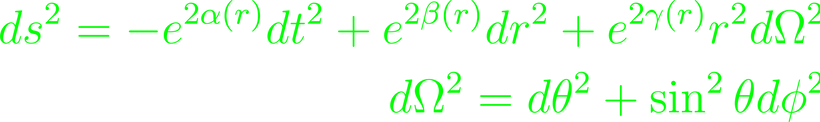
This ansatz assumes generalized functions for alpha, beta and gamma. As exponentials, they fit well into the radially symmetric ideal assumption and they don't have a time dependence. One could proceed with the calculations from here, though because of the degrees of freedom this system has, we can insert a step here to further simplify our system. Because the exponentials are just scaling factors at the end of the day, we could choose our radial coordinate to include the gamma-factor, so that it falls away. Since neither alpha nor beta are explicit, this won't really play into those part of the definition. Similarly, using the ln() function, the transformation factor can be absorbed into the beta exponential as well.

From here, the metric can be read off.

The calculations up to the Ricci tensor will be relegated to the exercise section of this chapter. To continue further, the Ricci tensor is set to zero, from which we obtain expressions for the exponential functions, which in turn will give a repeating factor, as well as be directly dependent on an as of yet undefined factor, which we will refer to as the Schwarzschild Radius. Application of these will give us a metric called the Schwarzschild metric.

This also gives the unique spherically symmetric vacuum solution (Birkhoff's Theorem).

Fix up the Metric

Clearly, the Schwarzschild metric is only sensible to use when looking at gravitational sources with some mass, otherwise the metric will be flat. However, the radial factor in the denominator might be a little concerning, is case it were to tend towards zero. At zero radius, the first factor would tend towards infinity, for r = 2GM the second would. Knowing manifolds, the fact that some slopes tend towards infinity itself isn't necessarily a problem, but it very well could be. Whether or not this turns out an honest singularity, or one that can be circumvented (or ignored, in our case) is to check whether the scalars diverge at those points as well. Our current list of scalars include the Ricci Scalar, but also all Ricci and Riemann tensors where all indices are contracted. The latter case will show in this case, that r = 2GM is not an issue. Still, we know for a fact that the something happens around the Schwarzschild radius. To study this area of the metric, we consider radial null curves, i.e. the radial part, so we set the angles to constants, if the line element vanishes.

At r = 2GM the derivative diverges, meaning that the light ray never reaches this radius, but instead experiences asymptotic behavior. Conversely, we would never see an observer cross this boundary either, and evenly spaced light pulses would reach the observer in longer and longer intervals as they approach the Schwarzschild radius. From here, several attempts to "fix" the metric can be made.

One intuitive solution would be to find a coordinate for the time that forces moves more slowly along the null geodesics, so to force the position over the boundary. Such a coordinate is called a tortoise coordinate for its property of just being slower than the normal coordinate.

In this case, the tortoise coordinate r* is constructed to function below the Schwarzschild radius, since that is the section of interest for us. This eliminates the singularity at r = 2GM. The coordinates as they are make computation a little tedious, since now r* has a direct dependency of r. Instead we can introduce two new coordinates to circumvent this problem. v = t + r*, u = t - r*. These are the Eddington-Finkelstein Coordinates, that have the advantage of eliminating either of the coordinates, depending on whether the null geodesic is infalling (v constant) or outgoing (u constant)

This behavior falls in line with the Event Horizon of a blackhole. The hyper-plane at the Schwarzschild radius is locally regular, but functions as a point of no return. Particles can never cross it to escape to infinity. We have, in essence, found the radius at which our metric describes a black hole. This behavior can be charted using yet another transformation, in which the intent is to maxmially extend the Schwarzschild solution, i.e. eliminate the points in infinity that are introduced by the linearity of both u and v.

This changes the metric again.

This set of coordinates are called Kruskal Coordinates, which are advantageous for the many ways T and R become constants. They then are convenient to chart against each other which the results in a conformal diagram / Kruskal diagram (below, taken from Spacetime and Geometry, Sean Carroll).

The cross signifying the even horizon solutions splits the diagram into four regions. Along arrow convention these, region I is where the radius is greater than the Schwarzschild Radius. This is where our usual observers will move and exist. Passing the Schwarzschild radius into region 2 will plop the observer into the black hole. Crossing the other radius again into region IV lands the observer into what is usually thought of as a forbidden region. It mirrors the metric, but crossing into region I is impossible. Region III is what's commonly referred to as the inverse of a black hole, i.e. a white hole. The singularity is in the past, so the observable universe is emerging out from this singularity.

Black Holes

By the previous chapters we have not only seen what happens when singularities enter our metric, but also got us a good definitions for the more stringent ones that result in Black Hole behavior. All black holes are chiefly characterized by the existence of some event horizon, much rather than the existence of a singularity. The conformal diagram showed its function in separating the timelike paths from non-timelike paths, which characterize forbidden paths nicely. From construction, the event horizon can be thought of as a null hyper-surface, so generated from a collection of null geodesics (combinations of which also give null geodesics, of course). In the Schwarzschild metric, the event horizon took the form of the light cone approximating a null-surface, but that is a phenomenon dependent on the chosen coordinates. We seek a more generalized criterion to identify event horizons, given stationary and asymptotically flat metrics.

For this, it is useful to understand which conserved quantities contribute to black hole phenomena. These turn out to be mass, charge and spin. Charge in general relativity follows directly from Stoke's theorem and the relativistic Maxwell's equations, using the field strength tensor discussed during the transition from special relativity to general relativity. Similar to the classical application of Stoke's theorem, the charge is determined by a path integral over the volume element multiplied with the electric current. Since the electric current is derived from the field strength tensor alone, the charge is chiefly dependent of that quality, along with the metric, which directly gives the volume element.

The mass energy of the some asymptotically flat spacetime is derived from the energy-momentum tensor and the Killing vector field. From these, we can construct a "mass current". We have to take the Killing vector field into account, as the energy-momentum tensor only describes matter energy, and we have seen that this alone is not a conserved quantity. In this way, there can be found an analogous definition for the total energy of the system, though of course the definition of the current is not trivial as it was in the case of the charge. There are cases, even within the Schwarzschild metric, in which the current becomes trivial, which would of course spell doom for the integral, so even though intuitively this should work, a different approach might be in order.

The Ricci Tensor has the same order as the energy-momentum tensor and through the curvature, the mass of the system can also be determined. As such, a current using the Killing vector and the Ricci Tensor is also a valid description of "mass current". Since the Ricci tensor is not divergenceless, it definitely won't become trivial in any of our scenarios (asymptotically flat spacetime), unless the spacetime is perfectly flat, i.e. the system itself is fully trivial. Using some property of the Killing vector, the current can be written as follows

The Killing equation is also symmetric, so with some normalization, the mass of the system is expressed through the Komar Integral

Spin is quantified using a rotational Killing vector and doing more or less the same thing. The textbook definition uses R for this Killing vector, but I will refrain from doing that, for the sake of notation.

Charged Black Holes

Adding charge to the black hole basically overlays a Coulomb-potential over the problem. It is, of course, still subject to changes in spacetime, and the resulting metric is still spherically symmetric. Electromagnetic interactions however do not take place in vacuum, so we adapt the energy-momentum tensor. It now derives from the field strength tensor, and using its (anti-)symmetries gives the Reissner-Nordstrom metric

Where Q is the total electric charge and P the total magnetic charge. Note, that the inclusion of P assumes a magnetic monopole, something that Maxwell's equations forbid, so it can be set to zero in practical computations, in theory however, keeping it around is interesting just to understand the hypothetical, seeing as by definition, magnetic and electric fields affect the metric the same way. To arrive at expressions of the fields (functions of radius for symmetry reasons), just divide the square radius out of the charges, as expected of Coulomb potentials. It's also worth noting that the coordinates of the Reissner-Nordstrom metric have been chosen so that the rr-component of the metric is exactly the Δ defined in the metric, and the event horizon sits at Δ = 0.

This gives three domains to solve depending on

In this case, Δ is always positive, so the only singularity sits at r = 0, which means there is no event horizon for timelike radii. By construction however, timelike geodesics don't intersect r = 0, but are rather repulsed by it. This is a naked singularity, and it states that the total energy of the black hole is less than the contribution to the energy from the electromagnetic fields alone. Since this is an odd, unphysical statement, we usually reserve this to wrong hypotheticals.

In the opposite case, we can assume that the opposite of the previous case are (roughly) true. This feels better on first contact. The metric coefficient is negative within the two solutions at which r = 0 -> r*, and positive outside it, and r* mark singularities. These are null surfaces and function as event horizons as we approach them. The inner area of this ring area however functions as space, so this might reasonably describe a "wormhole", which is not very well documented as of yet, and currently conjecture beyond this theory.

If α = β, the solution is interesting, but complicated. It retains certain symmetries otherwise broken in quantum physics, but is eternally unstable, as the mass is balanced by the charge. By construction, two of such black holes will attract each other through the mass and repel one another through their charge. In sum, these effects will cancel exactly. Closer solution of this system will exceed the point of these texts and is probably better off getting one of its own in the future, with some forays into quantum-gravity.

Solutions of rotating black holes are tedious in all of their aspects, since we lose the spherical symmetry and have to settle for axial symmetry (around the axis of rotation) and a timelike Killing vector. Carroll doesn't give a full derivation of the resulting metric, so I won't either, under the assumption that it's too much work to do in a reasonable time-span.

This is the Kerr metric, and it's - frankly speaking - terrifying to me. Accepting that this is what we have to work with, we identify the constants. The mass M is defined by the Komar Integral and a is the angular momentum divided by M. Charge may be added to the metric through a simple transformation

The characteristics of the rotating black hole and the charged black hole are independent of one another, we won't lengthen the metric anymore than we already have, and just keep this convenient fact in the back of our mind.

The remaining Killing vectors are that of time and that of the rotational angle, which expresses the axial symmetry. The time Killing vector is not orthogonal to any hypersurfaces, including the constant time hypersurfaces. The metric is stationary, but not static. From the metric coefficient, again, three cases arise. If GM < a, then the singularity is naked again and turns out unphysical. GM = a, is again, even more complicated than it was for the charged, static black hole, so we won't get into it. For GM > a, we recover the negative disk along

Both r* will be event horizons once again and their solution follows the pattern of the Reissner-Nordstrom solution. Unfortunately, the event horizons are not Killing horizons, so there is a separate stationary limit surface within which remaining stationary is impossible.

The squared cosine factor is set to one for the outer event horizon, so the stationary limit surface is larger than the outer event horizon. In practice, massive particles (that is moving at below light speed) are dragged around along with the hole's rotation within the stationary limit surface.

Gravitational Radiation

Usually, the spacetime metric won't actually be as neat as we have so far assumed it to be. It also turns out that slight changes in the metric are important for some interesting observations within general relativity. To correct these assumptions, one has to apply some perturbation theory, which is long and arduous, but follows a relatively easy concept. No matter the metric, it can be decomposed into the flat Minkowski-metric with a (small) perturbation.

Technically, this approach is valid for any metric we know the solution to, but in this case, the notation is just convenient. From here, we once again aim to identify the equations of motion. The Christoffel symbols have a convenient form that doesn't make stuff much more complicated.

We'll skip the remaining computations until we get to the exercises. An issue here though, is that this decomposition doesn't necessarily create a unique coordinate system. It's possible to choose a different perturbation, but arrive at the same coordinate system. The solution to this problem lies in the maths of diffeomorphisms and gauge invariance. Explaining this in detail would require too much maths to do on the fly now. Suffice to say using diffeomorphism properties to at least establish a bijection between the metric and coordinates that is unique up to gauge transformation.

As perturbation theory complicates the Einstein tensor, it's useful to find some ways to simplify the problem before getting into solving the Einstein equation. A good way to do that is identifying the degrees of freedom and reducing the problem based on that. Metric perturbations are symmetric (0,2) tensors. It can be decomposed itself into a trace and trace-free component, so by elements, the perturbation can be written as

which can be directly written into the metric without needing to choose a gauge. The traceless tensor s will later turn out to describe gravitational radiation. The time geodesic written using the 4-momentum turns out as follows

And the 0-component gives the evolution of the energy. Since it only includes the inertial energy of the particle, it need not be conserved. To describe the time-evolutions following from the geodesics, one can define vector fields to generalize the expressions. We call them Gravito-Electric and Gravito-Magnetic 3-vector fields, for the way they interact with the vectors in the expression of the time evolution.

From here, it makes sense to calculate the Riemann, Ricci and Einstein tensors by the same components as h.

From the Einstein equation, then only a few of the metric components reveal themselves as true degrees of freedom. At this point, gauges may be applied. Choosing one called transverse traceless gauge, where we set the energy-momentum tensor to 0 helps in expressing gravitational waves. Because of the tracelessness and transverse property of the perturbation, an analytic Ansatz can be made for the perturbation.

C is traceless, symmetric, constant and purely spatial. For nonzero solutions, the square of k still has to vanish. Since the wave-vector is zero however, we can understand that as the propagation velocity being equal to light speed. From transverseness, the derivative of the perturbation is zero, so the wave vector must be orthogonal to C. We can then assume a form of C, where the diagonal is (0, a, -a, 0), and the counter-diagonal is (0, b, b, 0). The remaining entries vanish.

The effect of a gravitational waves on test-particles needs to be determined as ensembles of at least 2 (the motion of the particle would remain as it was initially due to adaption of the metric). Each pair of particles is characterized by their 4-velocities and a separation vector S.

For slow-moving particles, the 4-velocities can be put to unity and corrections may be ignored. We then only need to substitute in the transverse traceless metric perturbation for the Riemann tensor. The elements a, b in the solution to C completely generate the wave and inputting values for each gives dictates the distortion of space. a here generates a distortion with a "+" pattern, b one with an "x" pattern.

Working with sources of gravitational waves requires looking at the gravity-matter interaction, so the energy-momentum tensor can't be set to zero, unfortunately. The Ansatz for the perturbation then won't be as convenient. Instead one uses a "trace-reversed" perturbation

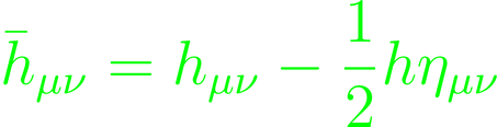
and chooses a gauge parameter with

This is called Lorenz gauge. The linearlized Einstein equation for this gauge turns out very simple, but it retains the d'Alembertian, which has yet to be defined. We use the Green's function to evaluate the d'Alembertian by using that the d'Alembertian applied to a Green's function gives the 4-delta function of its parameter. Then, the d'Alembertian of any given function can be written as an integral over the Green's function.

For computation, we choose the retarded Green's function. Evaluating this to the end gives a quadrupole form for the metric perturbation.

Cosmology

Concepts of general relativity find their application in cosmology. Underlying cosmology is the Copernican Principle, the assumption of homogeneity and isotropy of the universe, at least on a macro-scale (as this is obviously wrong on a micro-scale). Together, they imply that space has a maximum possible number of Killing vectors, or - in the superlative terms - that the spacetime is maximally symmetric. This description then gives us a good starting point to look at our own universe. The Riemann tensor for maximally symmetric n-dimensional manifold can be written as

with a metric of (- + + +) signature. Assuming κ > 0, the spacetime is described by the de Sitter metric. To arrive at the explicit equation, consider a hyperboloid for a 5-dimensional Minkowski space. Then insert the definitions of coordinates using spherical coordinates.

This gives a metric on the hyperboloid.

The anti-de Sitter metric can be constructed using the same method, but assuming that κ < 0.

Where dΩ is the expression in the round brackets of the de Sitter metric. It matches the metric of the 3-sphere. For κ = 0, we default back to the Minkowski-metric. In sum, we then have 3 maximally symmetric spacetimes: Minkowski, de Sitter, and anti-de Sitter. To identify which ones of these are useful, we can just use our assumption and have our tensors and scalars be dependent of κ. Over the Riemann tensor, we can solve the Einstein tensor and gain an expression for the energy-momentum tensor.

We use our ordinary matter and radiation, with vacuum energy with an expanding universe. As such, the expression for the energy density and pressure don't make a lot of sense in any of the maximally symmetric solutions we've seen, but they prove sufficient for locally unique solutions in the absence of ordinary matter or gravitational radiation. We then have to abandon the "perfect" Copernican principle. We retain spatial homogeneity and isotropy, but have a non-trivial time-evolution of the universe. Each timlike slice of the universe then is maximally symmetric. Doing so introduces the Robertson-Walker metric.

Applying the metric to the perfect fluid model gives again the conservation of energy equation, which we need especially for macroscopic considerations.

The way the density scales with a reveals the dominating component. For matter-dominated energy, the density falls off with an exponent of -3, with radiation-dominated energy, with -4 and with vacuum-dominated, the exponent vanishes. For the einstein equation, this helps in eliminating the second derivatives and give the Friedmann Equations.

Together, these equations describe the expansion of the universe. An expansion in that way of course has some consequences for observing events. One of these is the redshift phenomenon, where an emitted photon's frequency will be observed as lower as the distance it's traveled expands.

Similarly, two stationary objects will appear to move apart over time. This can be a problem over large distances (larger than the Hubble radius), since we are operating in timelike slices, so time and space comparisons aren't technically allowed. The redshift is used to cheat over small distances, by expressing it as a velocity.

where H is the Hubble radius. For larger distances, we should use the luminosity distance, that takes into account the luminosity of the source and the flux measured by the observer. From there, it's mostly geometry. Since the expansion is not isotropic, then there is also the phenomenon of gravitational lensing, the details of which I will hash out in the Exercises.