Yang-Mills Thermodynamics
Semisimple Lie Groups SU(N) (N ≥ 2)
This is a special case of non-Abelian gauge groups, which is especially relevant to characterize the fundamental forces for at least the standard model, and must set the motivation for alterations to it. SU(N) in its fundamental representation consists of a product of unitary N ⨉ N matrices with positive determinants, which are themselves associated with linear, special unitary transformations of a complex vector space. From previous entries, we should know both that SU(N) is a continuous Lie group, and the definitions of Lie groups. For the intuition of the following, Lie groups should be thought of as differentiable manifolds. Elements of a Lie group may be expanded about the unit element as
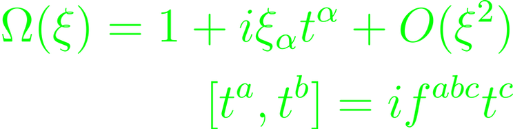
with traceless and Hermitian generators t, structure constants f, and some distance parameter ξ from unity. This distance may be represented by the exponential of iξt, meaning an infinite series of infinitesimal transformations. The generators span a vector space, with dimension N² - 1 for SU(N). In the following, we note the Lie algebra of a Lie group G as g.
SU(N) is semisimple insofar that its Lie algebra su(N) is a direct sum of simple Lie algebras. See the course on fundamentals of algebra for a more rigorous definition of simple algebras. Within physics, it's convenient to map the group action of SU(N) onto a space determined by the spin properties of a particle, using a representation of dimension 2J + 1 where J is the total spin (half integer, starting with 0). The Weyl theorem implies that this representation is completely reducible. For irreducible representations r of SU(N), their generators can be normalized down to a coefficient that is consistent with the structure constants.

In Yang-Mills theory, the standard representation of a Lie group is spanned by the generators, i.e. its own Lie algebra, so that the adjoint representation are given directly by the structure constants with maximal dimension.

with a representation-dependent constant C. For SU(2), the generators can be normalized into the 2D fundamental representations built through the 2-Pauli-matrices.

For later use, define the center of SU(N)

Gauge Connections and Gauge-Invariant Objects
The Lie-algebra valued gauge connection in the standard fundamental SU(N) representation is defined through real functions of space-time coordinates A. For a good generalization of the transformation law of SU(N), A(x) needs to transform inhomogeneously.

Local densities are functionals of A and are invariant under the SU(N) transformation, so A should transform homogenously in the fundamental representation. The gauge invariant quantities can be obtained through the trace of exponents of A. The field-strength tensor F is defined as its usually defined, and separately treating the inhomogeneous terms.

The Lie algebra then traces over local polynomials of this field strength tensor, and is gauge-invariant. Homogeneously transforming adjoint objects have covariant derivatives that transform in the same way.

It's convenient to adopt a gauge coupling constant of whichever definition for the trace over two generators, and including it into the gauge field definition as well to cancel it for the invariant portion, but retain them in the appropriate exponents in the inhomogeneous portions. This fixes the field strength tensor and with it, the fundamental Yang-Mills action.

The validity of Yang-Mills theory will become clear in its perturbation theory. The gauge field configurations are associated with topologically nontrivial mappings of boundary of 4D spacetime, which can be represented by a 3-sphere. The group manifold S3 is a subset of SU(2). The lower bound of the action is given characterized by the winding number (or topological charge k). Perturbation theory ignores topologically nontrivial field configurations.

Through invariance und a translation of spacetime, four conserved currents exist, which in turn leads to conservation laws. Euclidean rotations for (anti)self-dual field configurations extends these conservation laws in terms of electro/magnetic fields. This guarantees that (anti)self-dual Euclidean gauge field configuration of finite action will not propagate for a lack of energy-momentum, regardless of underlying metric signature. This property is inherited to quantities derived by averaging over this non-interacting (anti)self-dual Euclidean gauge field configuration

Spontaneous Gauge-Symmetry Breaking
A smooth curve in 4D spacetime has a "Wilson Line" along itself, defined through an exponential.

with a path-ordering operator P. It's an element of SU(N). If C is a closed loop, then {x, x} of the gauge field A locally transforms under adjoint representation. This results in a "Wilson loop". Shifting the base-point of the curve shifts the group element that determines the gauge transformation Ω.

is gauge invariant. The average of these quantities grows with the area of the contour of the curve.
Spontaneously gauge symmetry breaking can be introduced by non-invariance of the ground state under gauge transformation. Assume the existence of a scalar field ϕ and an extended ground state estimate. This means that the theory is equipped with a gauge-invariant potential V(ϕ), or an appropriate boundary condition. The scalar field ϕ transforms under an appropriate representation of SU(N). If ϕ is charged under the adjoint representation, the minimally extended Yang-Mills action is

The field modulus |ϕ| has a constant ground state expectation, and so the field can be decomposed to said constant expectation value with a perturbation. It can solve the classical Euler-Lagrange equations of motion, following from the Yang-Mills action. The resulting energy density is constant, thus proving the assumption valid, though the constant field-term may break gauge symmetry. Generally, its direction in su(N) can be chosen to be parallel to some generator. Neglecting the perturbation leads to the following Lagrangian

Commuting generators hint toward modes of A, which propagate as massless gauge-field excitations with 2 polarization states. There are exactly as many of these modes as SU(N) has ranks, which is N - 1. Symmetry-breaking generators get a mass, propagating with three polarization states.

These configurations can be developed toward finite actions, static energy, possibly per spatial line element. The first case is fairly natural in 4D Euclidean spacetime. The other two cases require non-trivial dependece of ϕ₀ on the spacetime. A Lie group that can be broken down to a subgroup H by a non-vanishing groun-state estimate, ϕ₀: G → H. ϕ₀ is invariant under gauge transformations emerging from H, so G/H consists of elements that either satisfy all three cases, or see the lower-dimensional cases vanish at infinity. Choosing the boundaries of n-dimensional real spaces as n-1 spheres, the gauge field approaches a pure-gauge configuration with an action density that vanishes at infinity.

For finite actions, the group elements Ω may cover the entire group manifold of SU(2), which is a 3-sphere. The set of all classes in Hom(S3 → G) is the "third homotopy group of G". Families of maps associated with the group elements are pairwise non-intersecting, the minimal-action field configurations with asymptotic behavior of this type are stable, and solve the field equations.
For the static energy cases at infinity, those points at which ϕ₀ induces vanishing static energy density or static energy per line element. Either case is parametrized by 3- or 2-dimensional unit vectors. The stable field configurations lead to Hom(S2 → G/H) or Hom(S1 → G/H), neither of which is trivial. It implies that closed curves are not contractible on G/H. The associated topological stabilized field configurations of Hom(S2 → G/H) are finite-mass magnetic monopoles, where "charge" refers to the 3D charge described through the unbroken U(1) gauge group. It's topologically invariant and emerges from Hom(S2 → G/H) = ℤ. The fundamental group being nontrivial should be familiar at this point. Its topologically stabilized field configurations are infinitely long, magnetic vortex lines with a finite line density of mass. The 2D charge is topologically invariant.
Gauge Fixing in Functional Integration
An element of the S-matrix is determined by a functional integral with a Yang-Mills action functional S[A]

The integration measure is taken over a system of an uncountable number of degrees of freedom in 4-D spacetime, with an asymptotic gauge field configuration. The gauge copies need to be identified and factored out of the product before applying the integral. In a Lorentz-covariant regime, only specific points in the gauge orbit are allowed:

with an arbitrary su(N)-valued, gauge-invariant Lorentz scalar function K(x), group elements in adjoint representation R[ω] and ω-dependent shifts f[ω]. The measure is gauge-invariant, so the YM-action in the integrand is as well. This allows exchange of mutually invariant variables without introduction of additional factors, which also extends to the definition of the covariant derivative. The functional determinant of the operator can be written as a Gaussian functional integration over complex Grassmann scalar-fields.

The kinetic component of the (fermionic) Grassmann-field c carries the wrong sign in the action, which implies so-called "ghost fields". Each ghost loop then requires an additional factor of -1. The gauge transformations are only integrated over as some factor, that can be ignored in qualitative reading of the functional integral. The functional integral has no dependence on K(x), and so its computation can be included as a factor with dependency of a "weight functional" F[K], which can be chosen almost freely.

The modified action sees contributions to cutting rules completely being based on unphysical phenomena canceled. This whole procedure is in reference to the Faddeev-Popov procedure. It doesn't fix the gauge completely, and arises from partial gauge invariance.
One-Loop Running of Gauge Coupling
Computation of the running coupling constant at one-loop level is stuff of QFTII, but complicated enough to always merit repetition. In the Yang-MIlls perturbation theory, the free field will augment the gauge potential using this coupling constant. For this, define the Feynman rules in momentum space.

with k, p, q four-momenta of the external lines. The usual integral is taken for computation of a function in the momentum space. It gains a symmetry factor l, the inverse of the number of possible ways of interchanging components without changing the diagram. Each ghost loop carries a factor of -1. The non-interaction hypothesis between the bare-connected n-point functions G and its renormalization condition at momentum scale μ is expressed via the Callan-Symanzik equation. Dependencies on these conditions that don't know about the renormalization points must cancel these dependencies, by construction, using subtraction. Renormalized n-point functions carry μ-dependencies via the coupling-constant, wave-function subtractions, and possibly explicitly.

Z and g are dimensionless and are not themselves affected by the scaling of the renormalization. The only explicitly renormalized parameter is g. At one-loop level, a three-point function with gauge fields as external legs and the Yang-Mills β-function is

Consider a 4D-integral over loop with 4-momentum l with Lorentz-scalar D(l)

This integral is antisymmetric under l → -l, for ν ≠ μ, meaning that it vanishes for integration over the entire space. For construction of second-rank tensors, the integral then needs to be proportional to the metric tensor. Via Wick-rotation:

Once the Wick-rotation has been performed, eliminating UV-divergences without breaking gauge-invariance, is done through regularization by continuation of physical dimension of spacetime to a 3.x spacetime.

We use the Feynman method, stating that for B > A:

A loop integration over p may be performed over P. With these methods, the subtraction constant of the β-function can be determined. For this, only the coefficient of the poles are relevant, not the exact renormalization condition, and so the Feynman rules may now be applied. The integrations of the resulting terms of all diagrams of the same genus at 1-loop level yields a bunch of constant factors, which makes up the renormalization counterterm of the β-function.

Because of the contributions of diagrams with external fermion legs, these two expressions do not approach by just setting n → 0. For small enough n, the terms become negative, meaning that the coupling constant becomes smaller, as the scaling of the scattering process increases.
Free-Particle Partition Function
A path integral over the field configurations gives a representation of the thermodynamical partition function. The resulting Euclidean formulation of thermal field theory enables topologically nontrivial solutions for equations of motion, which in turn enables nonperturbative theories for the thermal ground state at high temperatures. Effective excitations in Yang-Mills theory requires a momentum space formulation to discern quantum fluctuations from thermal effects. The thermal ground state sets the scale of maximal resolution, so it needs to be expressly identified for a complete theory.
From the Minkowski metric, the path-integral representation mapping onto the space of field configurations itself includes a Gaussian integral, for which the expression can be normalized without paying too much attention to the resulting factor. Recover from that, the partition function Z.

This implies a periodic solution. It's a familiar equation, usually solved using something akin to variable conjugation in both time and space. From this arises the Matsubara frequency, and the Fourier transform of a differential operator D.

Extend the modified ideal gas law to these equations via the logarithm of the partition function.

The root term is in reference to the vacuum fluctuations. Free theories on flat, 4D spacetimes are defined to have no vacuum energy, so contributions with linear dependencies of vacuum fluctuations, and those without x-dependence, can be set to zero. For small a, the thermodynamical pressure P can be expanded to a completely time-dependent expression. Solving it requires a solution of the Riemann-Zeta function (for z > 1)

As the derivatives of I(a) with respect to a² diverge at a = 0, higher derivatives of P(a) than those of second order are not defined at a = 0. Instead, a resummed expansion should be used, though it modifies the integrand of I(a), which can then be split into an infinite sum and remainder. The final logarithmic contributions, and odd powers of a are the source of the nonanalycity of P in a² around a = 0.

The imaginary time in the finite-temperature field require integration over the Matsubara frequencies. This method makes quantum fluctuations impossible to identify. As mentioned, quantum and thermal effects are independent from one another, so the theory needs to be reformulated via the imaginary time propagator. The thermal topological field configurations contributing to the ground state can unfortunately only be expressed through imaginary time, while the formulation of thermodynamics of effective excitations on different time-integration contours in the action is inconsistent insofar that the partition function is only ever defined on a single spacetime over the entire theory.
The connection between imaginary and real-time formulations lies in the one-loop diagram. In imaginary time, it can be represented by a frequency sum of analytic functions. It may be set equal to the integral over a spatial momentum expression via a contour integral.

The factor in the integral has simple poles at p₀ = 2πnTi. C is assumed to be a set of closed circular curves with r < πT, and centered around the poles. The contours can be deformed into two lines parallel to the imaginary axis. The clockwise rotation of the contour of the sum at T = 0 to the real axis circumvents the poles. For T > 0, the contour must be closed by a semicircle over the infinite right half-plane.

The right side of the final equation is the real-time propagator of the scalar field in momentum space. It splits into temperature-independent parts and a part in which the thermal fluctuations are Bose-distributed on the mass shell. This description currently sees no momentum transfers in diagrams such daisy diagrams, so an additional formalism needs to be introduced, making sure that the contour for the integration is more precise/elaborate. The δ-function is replaced by a function describing the physical energy spectrum of intermediate states at fixed spatial momentum. This "spectral function" expresses the imaginary part of the self-energy, and erases the mathematical inconsistencies.
Perturbative Loop Expansion
In 4D Yang-Mills theory, perturbation theory generates an infrared cut-off for magnetic screening, that is too weak for convergence of thermodynamical quantities. The nontrivial thermal ground state on the propagation and interaction is affected by this effect even at higher temperatures. It's constructed of gauge field configurations, approximated by the perturbative expansion and will add mass to the effective theory. The apparent gauge-symmetry breaking is independent of a small coupling assumption. It leads to a fast convergence of loop expansions, evading the perturbative infrared problem. Motivation for the approach is taken from replacing the renormalization scale by the temperature at asymptotic freedom.
Matsubara frequencies of course dictates the modes in terms of mass. The vanishing ones express massless 3D gauge modes, while the rest are associated with the massive ones, which behave linearly with temperature. Massless 3D modes are given by the effective action, and can be expanded to four dimensions via perturbative matching. It contains some free parameters, in form of coefficients

The consideration for three dimensions is less computationally intensive, but requires truncation at low values of M, and a convergence behavior at nonzero M, to match the 4D behavior. In 4 dimensional perturbation theory, the mass-scale is generated by the gauge coupling constant g, The momenta (i.e. powers of g) of order T are categorized into hard, soft and ultrasoft hierarchy for the modes. Integrating out the momentum scales starting from hard and working down the orders, will experience screening of softer modes by the harder ones. The Interaction monomial I of the YM-Lagrangian is hierarchically smaller than the expectation value K. The magnetic modes experience weak screening. K~g⁶T⁴, I = g⁶T⁴, so K ~ I. Starting at sixth order of g, the loop expansion of the pressure (sans free energy) contains contributions otherwise not determinable in perturbation theory. This describes an effective Lagrangian density. On the other hand, below this order, YM-theory is considered somewhat incomplete. Matching of the 3D coefficients to the full theory happens perturbatively.
To address the inherent global symmetries, take the Polyakov loop as a central field variable in the 3D effective theory. It's a Wilson line of the gauge field along a compact time interval, and transforms under 4D gauge transformations induced by the native group elements. As an element of the center group, its elements are distinct, and commute with any SU(N) group element.
For SU(2), the perturbative definition of the gauge field without absorption of the fundamental coupling g is defined through its Wilson line on a Euclidean background

with the path-ordering operator P. The gauge transformations are associated with a center jump along the time-axis. Through the invariance under singular, periodic gauge transformations induced by the group, the YM action density partition function is also invariant.

This remains true for all SU(N) under the same generalizations of the center jump. This is a global symmetry. The Polyakov loop in its totality can be considered an order parameter for deconfinement, associated with the free energy of an infinitely heavy test "quark", transforming under the fundamental representation of SU(N). This is somewhat problematic, as it can be constructed to have infinite free energy, and so far no mechanism is included to stop the particle to gain infinite mass as well. This should be rejected as a test particle in a thermodynamical system. Outright rejection should categorically apply to isolated heavy quarks - it's only allowed to exist in a compound state with an antiquark, in which the gauge charge is completely screened at long distances. For Dirac fermions and its standard action, the gauge-field component is gauge-rotated into the one-direction of the Lie algebra, so that the heavy test-charge is located at spatial origin. The density is not in itself gauge-invariant. Under the effects of the full partition function, the thermal YM and static test-charge must be related to an expression invariant under smooth gauge transformations.

As Z should be finite, the vanishing of the average indicates that the electric and global center symmetry of the effective 3D theory remains unbroken, and the test-quarks are confined. If the average does not vanish, the N-fold center degenerate entails a finite force. This is the deconfinement scenario.
Instantons & Multiinstantons
Finite action of solutions of Euclidean field equations in Yang-Mills theory saturates the bound determined by the topological charge of the homotopy group Z. Z is either the charactersitic group with index 3, for pure gauge theory, or with index 2 for the adjoint Higgs model. The former results in a mathematical construction of instantons, the latter for magnetic monopoles or dyons. In the deconfined phase, these instantons appear in their periodic incarnations, called calorons, responsible for the emergence of a thermal ground state and stable magnetic monopoles.
For SU(2), the construction of the simplest instanton (|k| = 1) on ℝ⁴ and |k| > 1 is derived from the topological current and the decomposition of the YM-action. The resulting closed-form solution is a gauge-transformed version with the nontrivial topology at the center of the action density. SU(2)Π₃(S₃) has topologically stabilized finite-action solutions. This can be shown using the gauge invariant current
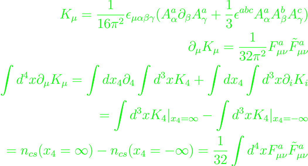
where n are the Chern-Simons numbers. These are the charge of CS-current on the time slices at infinity and describe the behavior at, along with of the invariance of the topological charge (Pontryagin index) under smooth, spatially localized deformation away from the boundaries. The Euclidean YM-action can be decomposed into a topological invariant term and a positive definite, non-invariant term. The minimal action is reached for a vanishing non-invariant term. A regular gauge-field configuration has finite action if it approaches a pure gauge. For Pauli-matrices τ, unit quaternions σ and t'Hooft symbol η. η is self-dual, anti-self-dual and antisymmetric.
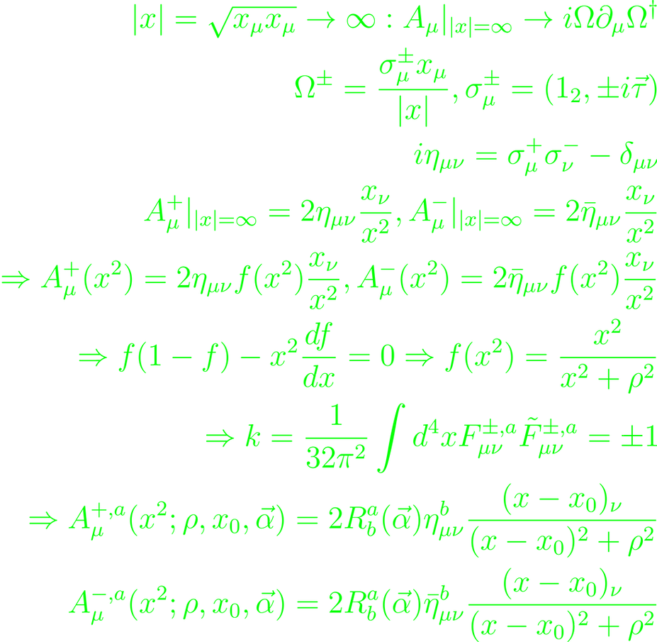
for |k| = 1, eight free parameters emerge, spanning an 8D Riemannian manifold called a moduli space. The solutions decay as |x| → ∞, so their topological charge is picked up by surface integrals of the CS-current over a 3-sphere with infinite radius.
Using the conjugation of the gauge fields as a gauge transformations introduces singularities at the origin, by which the invariance of the YM-action becomes visible. The saturation of the action at the |k| = 1 bound is fixed at the anti-self-dual gauge-field level. These can be narrowed down by using generalizing the boundary condition to higher topological charge moduli |k|.

Evaluated straight-forwardly, the configurations will turn out to be generalizable through multiplication with constant SO(3) matrices. The gauge-field configurations are then globally oriented in the Lie algebra, so that each |k| = 1 (anti-)instanton contributes one unit of topological charge with |k| = n, oriented the same way in su(2). These periodic configurations of the Euclidean formulation of the finite-temperature Yang-Mills theory will create calorons on the trivial holonomy. These configurations are generalizable to SU(N).
Assume a traceless, antihermitian gauge field. This will restore tⁿtᵐ = -1/2 δⁿᵐ, and make sure that the coefficients in the gauge field are real. It also eliminates the imaginary coefficients in the field strength tensor that would have decorated the commutator.
For k > 0 in SU(N), the self-dual gauge field emerges from the kernel of a 2k ⨉ (2k+N) matrix Δ⁺ = A + BX, where X = σᵢ⁺xᵢ and A, B (2k + N) ⨉ 2k matrices. Δ⁺Δ needs to be invertible and commute with the quaternions. Let V be the kernel of Δ⁺, then

A and B should be sufficient to generate all charge-k self-dual SU(N) configurations. The way to obtain all self-dual gauge-field configurations for some topological charge k at finite action is the ADHM construction.
The ADHM construction can itself be generalized to instantons on the 4-torus T4. For this, begin at SU(2), so to ignore gauge coupling, and the factor of -i into the gauge fields, so that the field potential ϕ follows the schema of the typical Lagrange density (up to a factor of -1/g²). Since ϕ ≠ 0 introduced a breaking of gauge-symmetry SU(2) → U(1), to consider Π₂(SU(2)/U(1)) = Π₂(S₂) = ℤ suggests topologically stabilized, static configurations with minimal energies for each topological sector. The field equation for the model become

Which can be simplified to the spatial dimensions if the solution is assumed to be static.

With some real scalar functions H, K which can be transitioned into solutions of the self-duality equations for the gauge-fields. This eventually results in differential equations of second order

This fixes the expectation at spatial infinity. An abelian spatial field strength should exist, which is associated with the magnetic charge of the static solitonic configuration. In the unitary gauge, this field strength tensor reduces to the usual U(1) expression, so fixing it to the magnetic field strength, This will derive the magnetic charge gₘ as a dual quantity to the gauge coupling g, along with the mass of the magnetic monopole, which vanishes as g diverges.
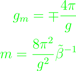
This is a sensible observation, seeing as the scenario would see a vanishing magnetic moment as well. This is in contrast to the Dirac monopole. This configuration has holonomy with its spatial Polyakov loop at infinity.

The BPS monopole with |k| = 1 represents the caloron configuration with trivial holonomy. New solutions are generated through symmetry of the Euclidean YM-action under spatial translation and global phase changes.