Category Theory
Category
When talking about math, one can either work from the direction of set theory, the way it's usually taught, which generally begins with a specific approach and abstracts it until it's the "correct" level of abstraction. Alternatively one can work from the direction of category theory, which starts very abstract and specifies until all the constraints have defined objects of sufficient specificity. Topology for example errs on the side of category theory, and my love for it might translate into interest in category theory. I want to at least check it out.
The definitions of basic category theory, already suffer from the general problem with category theory: It's non-specific, but complicated. A category C has a collection of objects (Obj) and arrows (Arw) and assignments mapping them onto one another as follows

For convenience, we take capital letters to be objects, lowercase letters to be arrows. Composition of assignments work as they do usually, along with basic traits such as associativity. For f: A → B, g: C → D are composible exactly if B = C to an assignment g ∘ f: A → D. There can be an arbitrary number of arrows between two objects A, B in C. The arrow class C[A, B] is the set of all such arrows. In literature it's also often referred to as the Hom-Set. Take objects N, M, L with arrows f: N → M, g: M → L, h: N → L. Here, g ∘ f and h map from the same object to the same object, but they don't necessarily have to be the same. They are a parallel pair. If they are the same, then the diagram commutes. Imposing some structure on a set and its arrows will define implicit rules, if one were to take the arrows as the abstracted versions of operators. These can have a number of arguments, and then this structure should be familiar to the reader as imposing an algebra onto a set.
One such structured set are the monoids (Mon). A monoid is defined as a structure (R, ⋆, 1) with a set R, a binary operation ⋆ on R, and a nominated element 1. The imposed algebra is (r ⋆ s) ⋆ t = r ⋆ (s ⋆ t) and 1 ⋆ r = r = r ⋆ 1 ∀ r,s,t ∊ R. These laws are recognizable as associativity and the identity element (usually for multiplication, so it's common convention to omit the operation symbol). Monoid morphisms should retain the structure of the monoid, so they are automatically injective. These are automatically bijective, so the direction of the arrow shouldn't matter here. Obviously linking several monoids with arrows will lead to situations where the order of application matters. With the identity arrow, this completes the Mon as a category with monoids as objects and monoid morphisms as arrows.
Because of the retention of structures of the morphisms, it's often valid to use the equality of arrows onto a known (third) object to justify the equality of objects. This is most often done through diagram chasing, which uses the fact that a diagram commutes to set arrows, or composite arrows equal to one another. If it's known that some cells commute, then by extension, other cells must as well. As a diagram, it's often somewhat trivial, seeing as the objects are already sorted in such a way that it doesn't appear more than once anyways. Whereas through injectivity of the arrows, the monoid morphism is defined, if the arrow is surjective, it defines an arrow called epic. It's the parallel to the monic structure in all other regards, except that it imposes a different algebra. The properties "injective" and "surjective" are really more approximations of the relation, rather than well defined terms. They are appropriate in the context of arrows as operators, not necessarily when considering categories as such. Instead, consider a pair of arrows between A, B so that r: A → B, s: B → A, r ⋆ s = 1. These define s and r as a section and retraction. By construction, each section is monic and each retraction is epic. Instead of describing them in terms of injectivity or surjectivity, these two properties are prescribed to arrows as split monics and split epics respectively. Of course there exists arrows that are both monic and epic. These are bimorphisms. If we keep in mind that by retention of object structure one can also define an isomorphism through bijectivity, then a hierarchy of arrows emerges.

If all bimorphisms of a category are also isomorphisms, then a category is considered balanced. The order in which monics and epics are applied between objects decides, whether a cell of a diagram commutes, as such their role in diagram chase is central.
Special objects in a diagram are those, which are at either "end" of a diagram. Depending on whether the arrow is emitted from the end, or it disappears into it, this is a limit or a colimit (in a categorical notion). What follows are examples of these types of objects in a diagram.
The Initial and final (terminal) objects are the limit / colimit, where each object A in the diagram has a unique arrow emitting/ending in it. It is, in a way, the most naive (co)limit construction. The shape of the diagrams organizes these objects as left / right universal solutions of a shape.
Products and coproducts emerge from the definition of a cartesian products of sets. This will pair up the elements a ∊ A, b ∊ B of both sets into elements of the product (a, b), but with that comes the "projection" as an arrow that associates the pieces of (a, b) back to a and b. Obviously. One could choose to sort these elements back to their sets of origin. The dual arrow is the disjoint sum of the sets, defined by (A × {0}) ∪ (B × {1}), which are also known as the embeddings. To get to a good idea of the initial and final objects, we should take a look at a full edge of the resulting X-shaped diagram. An initial / final object to several arms of a diagram is called a wedge, or more specifically a cone / cocone. A product / coproduct of a pair of objects A, B is a wedge X with projections / embeddings pointing to both, for which all other wedges (with arbitrary arrows sharing the same direction) have a unique arrow (mediator) pointing to X. A wedge can be both the product and coproduct for two objects. If there are several products / coproducts for the same objects, there are connected by unique isomorphisms that commute in the diagram. The cartesian product and disjoint sum both have group operator properties in Set.
Equalizers and coequalizers are initial / final objects emerge from parallel pairs of arrows, i.e. two arrows that trace the same path in a diagram (direction included) from the objects A to B. Take some object X with an arrow h pointing at A, where both arrows composed with h are equal to one another. A parallel object can be defined with an arrow h' pointing from B to X. Given these definitions, the equalizer / coequalizer is the arrow k (or k') to / from the object S which makes f and g equal in composition, and for every object X, the unique mediating arrow connecting X to / from S has the property h = k ∘ m (or h = m ∘ k'). Because of the construction being very similar to a doubled section / retraction, the equalizer is always monic and the coequalizer is always epic. Parallel pairs f, g from A to B with objects S, T a pair of equalizers to A / coequalizers to B, then the arrow l: T → A will equalize f and g through f ∘ l = g ∘ l and there has to be a unique mediator m: S → T. Similar for the arrow k: S → A and its mediator n: T → S. At the same time l can be taken to make the parallel pair equal, so that it doesn't matter which arrow is the equalizer and which one makes equal in construction. This implies l = k ∘ m ∧ k = l ∘ n. The mediators are an inverse pair of isomorphisms. We call S and T uniquely isomorphic. The parallel construction over the coequalizers functions analogously.
People who have done higher analysis should have encountered pullbacks and pushouts, but these originate from this corner of category theory. First construct a commuting square for objects A, B so that the wedges with X and C with arrows pointing away from X and towards C (or the other way around for the complementary). Take a wedge object S with the same properties as X will have a unique mediating arrow from X to S (or the other way around). If the square with S (instead of X) is a pullback / pushout and the arrow k: S → S endomorphic, while the resulting triangles commute, then k is the identity. The construction to show isomorphy of two pullbacks / pushouts is analogous to that for the (co)equalizers.
We have so far spared us the work for exactly half of the definitions, because of the way in that the diagrams were constructed. This can be made specific by using what is called the opposite category, which will turn around all arrows. It also swaps monics and epics, as well as final and initial objects.
Functors & Natural Transformations
The functor has appeared to me in the context of programming before, and I must admit that at the time I didn't really care enough to look at how exactly it's defined. They serve to compare objects, since looking too closely at an object itself is somewhat against the point of category theory. Take a pair of categories Src -> Trg with two assignments, one sending objects to objects (A -> FA) and one sending arrows to arrows (f -> F(f)). We define a covariant functor composition (Co) as preserved, if the arrows between the objects in both categories behave the same, then the compositions of the arrows retain their order. In the contravariant case (Contra) turns the arrows around in the composition. Note, that for both cases, the arrows are preserved.
In practice, a functor can be as simple as mapping an object to its parent set, and each arrow to its parent function. This is an example of a "forgetful functor", since information is irreversibly lost after application. Most easy constructions of forgetful functors are covariant.
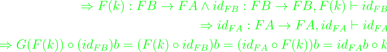
"Hom-functors" are also on the simpler side, but more important for future definitions. Let K be an object of some arbitrary category C and for each object A, there exists an arrow set LA = C[K, A] (RA = C[A, K]). The object assignments C -> Set, A -> LA (A -> RA) send C to the category of sets (assuming, the collection isn't too large to be a set). This actually also defines a pair of functors, sending the arrows of C to L(f): C[K, A] -> C[K, B], r -> f ○ r (R(f): C[B, K] -> C[A, K], l -> l ○ f) respectively. These are considered covariant (contravariant) hom-functors. To verify that this pair of hom-functors exist, consider a pair of arrows f: A -> B, g: B -> C in C. Further, consider the arrows r: K -> A, l: C -> K with r ∈ LA, l ∈ RC.

Interestingly, different functors can have the same object assignments in a set. Take three different endomorphic functors ∃, ∀, I living in Set, sending a set A to its power Set. The functors on the arrows will map the different power sets between one another either covariantly or contravariantly. Let's take ∃ and ∀ to be covariant, and I to be contravariant. Let's note

∃ will give the direct image across f, I the inverse, and ∀ the dual complement of the direct image.

Recall the wedge used to describe the product of two objects. This definition only carries uniqueness up to canonical isomorphism. Either way, the product in itself defines a factor. Consider some fixed object R in C, and define the arrows p, q such that p: A ⨉ R → A and q: A ⨉ R → R. Construct two such products with the same fixed R in a way that an endo-functor connect A → B. The identity maps R → R, so the functor is implied to map F(f): FA → FB.
Some categories can only be defined (sensibly) through functors. For instance, consider U he upper component and L the lower component of C, all three of which are categories, but let's first assume L and U as the appropriate set. This defines a wedge that looks somewhat like a co-product (U ↓ L), where U: U → C, L: L → C. Each element in c has associated with them an object in the upper and lower component set, so that Uu → c → Ll. Arrows between elements c, c' in C imply arrows between the upper set element and lower set elements, thus cementing it as a proper category. The functors U and L are then thought of as defining the upper and lower component categories.
The comparison of functors is done by of natural transformation, i.e. identifying the assignment each component arrow must take to satisfy the functor. A number of assumptions can be retained for functors that can be connected by natural transformations. These transformations can obviously take the form of a function between sets, so some of these transformations are isomorphic. In such cases, the functors are considered naturally equivalent.
Generalized Limits and Colimits
For a generalized approach to limits and colimits, there is somewhat of a roadmap. One starts at a template, which defines the shape of the resulting diagram. For the time being, that will be a collection of nodes and edges, which at the diagram stage will be sorted into categories. The node will stand in for an object and the edges as arrows. Depending on the type of diagram, it's required that some cells commute.
When the diagram is finished, there are two posed problems. There's the blunt end problem and the sharp end problem. Which that is exactly, will depend on the diagram. For these problems there are solutions to be found, each of which is a specific object within the category, along with some collection of arrows to satisfy the problem. The solution of the blunt end problem will have all arrows eminating from it, the solution to the sharp end problem will have all arrows pointing toward it. Each solution will pass through a node called the universal solution via a unique mediating arrow. The universal solutions are the limits and colimits, specifically, the universal left solution is the limit.
Technically the template of a diagram alone can be as complex as it likes to be, so it makes sense to define different kinds of diagrams. The template of the first kind is a directed graph where each edge has a nominated source and target that are objects of the category. A category on such a template will automatically define a functor onto the sets of nodes and edges. For each path in a directed graph (treat paths of length 0 as just the starting node), the category Pth is the category of paths through the graph; it's objects are the nodes, and the arrows the paths through the graph.
It's trivial to conclude that a category can be viewed as a template, so technically most of the above could be applied onto a category in itself. Note the categories ∇ and C, where ∇ is viewed as a template.
is the category of ∇-diagrams in C. The objects in M are functors into C, with a natural transformation σ in between them, provided they have the same sources and targets. These can be combined through composition in the usual matter to produce another natural transformation. The ∇-diagram then is a functor from ∇ to C, whose objects are indexed by the nodes, and whose whose arrows are indexed by the edges of ∇. Composible triangles commute to satisfy the composition of transformations requirement. A parallel definition can be applied using ordered and pre-ordered sets. In the case of a pre-ordered set, there may be nodes which are greater or equal to all pair of nodes in the set, which will qualify it as directed.
For a ∇-diagram in C, a left solution is a C-object X with a family of arrows ɑ(i): X → A(i). Assume that for all edges e: i → j in ∇, the triangle induced through ɑ(i) and ɑ(j) commutes. The right solution is defined flipping the direction of ɑ(i), but otherwise leaving the commuting triangle unchanged. There isn't generally any relationship between the left and right solutions. The existence of a universal solution, where such a relationship will exist is not given, but if it exists, it's canonically isomorphic.
The left universal solution (the limit) for the ∇-diagram is some solution S → A(i) through the set of arrows σ(i), so that for all solutions (indexed by arrows ɑ(i): X → A(i)), the unique mediating arrow μ X → S creates a triange in X, S and S(i) which commutes. Flip all arrows for the right universal solution (the colimit).
Suppose there is a solution with two arrows θ, ψ: X → S for all i. Then by the commuting property of the triangle X, A(i), A(j) induced by the edge e: i → j, and the uniqueness of μ, one finds that ɑ(i) = σ(i) ○ μ ∀ i. This must be true for both θ and ψ, and so they are equal. The arrow from a solution to the unique solution will then be unique.
Take the ∇-diagram with two limits S and T with a unique arrow τ: T → S. The arrows σ form a limit and the arrows τ form a left solution. The composition τ(i) := σ(i) ○ τ with the mediator τ implies the existence of a mediator σ so that σ(i) := τ(i) ○ σ ∀ i. The endo-arrow ε = τ ○ σ is the identity on S. The inverse composition is the identity on T. The mediators are thus isomorphisms that are inverse to one another, and that universal solutions are unique.
The categories Pos, Mon and Top are special in that their objects are structured sets whose structure is preserved by their arrows. For each there exists a forgetful functor onto Set sending the object to its carrier and the arrow onto the carrier function. The functor is noted as U. In the following, the family of a graph's nodes is noted as 𝕀 and the family of edges 𝔼.
Assume A is a family of sets, indexed over 𝕀 and define a choice function a(·): 𝕀 →∪ A : a(i) ∊ A(i) ∀ i ∊ 𝕀. Note the set of all choice functions for A as Π A. The evaluation at i is ɑ(i): Π A → A(i), a → a(i) = ɑ(i)(a). Assume the template ∇ is instantiated by a diagram in Set A = (A(i) | i ∊ 𝕀), 𝔸 = (A(e) | e ∊ 𝔼). The thread is a choice function a(·): 𝕀 ∪ A, A(e)(a(i)) = a(j) ∀ edges e: i → j. The evaluation functions ɑ(i): A → A(i), ɑ(j): A → A(J) with e: i→ j implies (A(e) ○ ɑ(i))(a) = ɑ(j)(a). The triangle of evaluation functions and A(e) commutes. Through this triangle one can construct a commuting triangle for some arbitrary solution of the diagram. For a solution to be unique, the mediator needs to be defined through the usual means, i.e. through composition.
Each of the Limits in Pos, Mon and Top are constructed in a similar fashion, though taking the structure of the group into account. In the case of Pos, this is the ordering of elements (by way of pointwise comparison). Mon is a bit more complicated on account of its monoid structure. The arrows in Mon then are monoid morphisms that are isomorphic with respect to the monoid operation. The diagram in Set would have to be furnished as a monoid that would retain the structure. Such operation would always form a thread. Due to the inclusion of the identity another element, this operation is associative. The properties of the monoid operator implies that μ(1) = 1. Extra considerations for Top emerge from the inverse image. It will require a property of the mediator: μ(x)(i) = ξ(i)(x) for every arrow pointing from a solution to the 𝕀 indexed family of topological spaces ξ.
Adjunctions
At the point where a full lecture would usually arrive at adjunctions, a lot will have happened. As such, this cursory primer will likely be somewhat clumsy, but hopefully not incomplete. The adjunction is, in general, an interaction between two categories, considered Src and Trg. The definition can be done both ways. I'll omit one side, but no meaningful information should be lost regardless. Define two covariant functors F: Src → Trg, G: Trg → Src. F is the left adjoint of the pair, G the right. Write F ⊢ G. Compositions G○ F on Src create an endo-functor so that

η is considered the unit of the adjunction (ε the counit). Take the pair A from Src and S from Trg. From these three objects, create two sets of arrows: Src[A, GS], Trg[FA, S] in which each of the arrows has an inverse counterpart in the other of the two sets. We note these transposition assignments as # and ♭, so the complete data to form adjunctions becomes (F, G, (·)#, (·)♭). Technically there's a bijection requirement between (·)# and (·)♭, but in this construction it's automatically fulfilled. Best to remember it's there, but not to think about it too much. More interesting is the naturality requirement, meaning that both assignments have to be natural. The pairs of the form (A, S) are the objects of the product category Src \times Trg. Functors Q and P can be constructed to send (A, S) into both Src[A, GS] and Trg[FA, S] respectively. Note those to be subsets of Set. Naturality would require (·)# and (·)♭ to be natural isomorphisms between P and Q. Beyond the definition of the requirement, it implies arrows k and l so that k: B → A, l: S → T with the compositions G(l) ○ f ○ k: B→ GT and l ○ g ○ F(k): FB → T. Check this by commutating diagrams induced by the transposition assignments. In fact, the bijectivity of the transposition assignments implies their naturality, and vice versa. For the naturality, this whittles down the requirement to either of the assignments, each of which can be decomposed into an upper and lower condition.
(# ↑) (G(l) ○ f)# = l ○ f#
(# ↓) (f ○ k)# = f# ○ F(k)
(♭ ↑) g♭ ○ k = g ○ F(k)♭
(♭ ↓) G(l) ○ g♭ = (f ○ g)♭
There exist equivalences between these components. Use the construction for proving the implication of naturality, but set k to the identity on A and l to the identity on S. Every adjunction should satisfy the four conditions. From there, it can be shown that the upper condition of one assignment is identical to the lower condition of the other, reducing the number of conditions to check down to two.
Let's think about the arrow k: B→ A from Src, and construct the square this implies with the functor (G○ F)B and (G○ F)A. It does, if

Both the unit and the counit of any adjunction then are natural. Take some natural arrow f: A→ GS and apply # ↓, so that f# = (id ○ f)# = (id)# ○ F(f) = ε ○ F(f). This gives the dual equalities f# = ε ○ F(f), g♭ = G(g) ○ η. Set f = η and g = ε to gain ε ○ F(η) = id and G(ε) ○ η = id.
Using F Ͱ G between Src and Trg so that η: Id→ G ○ F, ε: F ○ G → Id are natural transformations, then they are unit and counit of the unique adjunction F Ͱ G.
A free (cofree) functor is one pointing from Trg to Src (opposite for cofree definition), which is often forgetful. The free problem is an attempt to turn all Src-objects into Trg-objects. A solution to this problem is an arrow f: A → GS comparing the two types of objects. The construction of a uniform universal solution follows the schema of η: A → (G ○ F)A for all objects A. Note that η is only an arrow at this point, not a functor yet, although it certainly can be. For example, using the nomenclature of previous paragraphs, the object assignment F with the unit η and transposition (·)# provides a G-free solution, and (G, ε, (·)♭) provides the F-cofree solution. We already know that in such constructions, the assignment F and G are necessarily adjoint functors.
All these were considerations for the covariant adjunctions. The same notions can be defined for contravariant adjunctions by choosing different categories to work with and reversing the arrows. A good pair of categories to check for this are Alg and Spc.
Modules & Lower K-Theory
With our quick glance at category theory done, I want to look at some topics in analysis and algebra that have passed me by in previous studies in the hope of closing some gaps in my understanding and extending some of my usual mathematical categories. I know of injective modules at least, but have never had them defined as such, and because I suspect there's a good number of concepts, I've looked for a book that does that in the hope that it'll provide a complementary approach to that of those math lectures that are a bunch of years in the past by now (I don't like to think about it, makes me feel old).
I'm using Algebra 2 by Ramji Lal for the next few weeks. Obviously, there's a lot in here that I've already used and should be relatively familiar with, so I'll skip around a fair bit. The last third of the book will likely hold my attention the most, seeing as the book starts at very elementary linear algebra and works its way through some fairly ubiquitous concepts. Let's take some definitions for reminders first though.
A left R-module is an abelian (commutative) group over G, with a map α from R ⨉ G → G that retains structure. R is some ring. Take some set M, then the question emerges, whether some unique R-homomorphism φ exists linking an R-module G with a map α from M to G, to another R-module H with a map β, so that φ○α = β. Such a solution is the free left R-module on M.
This homomorphism can be constructed for all finite sets through some binary operation +, some product · and choosing a map from M to R which vanish at all but finitely many points, along with delta-function characteristics. for two parameters. Note that every left R-module is a quotient of a free left R-module by the fundamental theorem of homomorphisms and the universal property of free left R-modules.
A module M over a ring R is an internal direct sum of its submodules, if M is generated by the union of its submodules and the intersection of each submodule with the union of the others is empty, or the for every nonzero element m of M exists a unique finite subset of distinct elements of the index set for the submodules, where the nonzero elements out of each submodule so that their sum equals m.
Such an internal direct sum of its submodules is trivially isomorphic to the external direct sum of the same by construction of the external direct sum. The distinction between the two then is somewhat pointless.
At this point we take in some of what we've learned about category theory and apply it to exact sequences. A left R-module P is projective if given an exact sequence

for a surjective homomorphism β and a homomorphism f: P→ N. A commuting cell (MNP) can be built through the construction of a homomorphism g: P→ M. Note that every free R-module is projective. The definition of the injective module is complementary for the sequence

Extending these sequences so that

with a projective R module, then the sequence splits, since the latter half is exact and there exists an identity map on P. Dually for an injective M. Corollary to this, a projective second to last node in a short exact sequence implies splitting (The same for the an injective second node in a short exact sequence). Because of the splitting property, the direct sum of projective modules are projective, the same for the direct sum of injective modules. Since free R-modules are projective, then direct sums of free R-modules are projective. Assume that a left R-module P is projective, then a surjective homomorphism β: F(P)→ P delivers an exact sequence: 0→ Ker(β) → F(P)→ P→ o. For P's projectivity, the sequence splits and P is a direct summand of F(P). Left R-modules then are projective iff its a direct summand of a free R-module. Of course this can be done recursively over a family of left R-modules and their projective external sums.
What follows here is probably not going to be important for me for a while, but I went ahead and read it anyways, partially because I noticed it working with the Grothendieck Group, which I have very little experience with. Use the free abelian group F the basis of which is the set of isomorphism classes of finitely generated projective left R-modules, along with the subgroup of F generated by elements of the type [P] + [Q] = [P○plus Q], where [S] is the isomorphism class of the projective module determined by S. The Grothendieck group of R is noted as K(R) = F/N.
Let P and Q be finitely generated projective R-modules. They are considered stably isomorphic if

Projective R-modules are stably free if they are stably isomorphic to a free R-module. This is not the same as isomorphy.
Note the coset [P] + N as <P>. K(R) is generated by elements of <P>, so each can be expressed as <P> - <Q>. As such, <P> and <Q> are equal only if P and Q are stably isomorphic. As such, <P> - <Q> = <P'> - <Q'> iff P○plus Q' is stably isomorphic to P'○plus Q. To put this into context, consider two homomorphic rings R and S. A homomorphism between them preserves identity by definition. Define: r· a = rf(a), r∊ S, a∊ R, then S acts as a bi-(S, R) module, and thus a right R-module. Assume a left R-module M, then S○plus M is a left S-module. We write it as f#(M). The properties of f#(M) follows directly from the action of the tensor product. K(R) is isomorphic to N, if every finitely generated projective module is free, and:

Semi-Simple Rings and Modules
Let's pick up where we left off. We are now familiar with left R-modules, and submodules. Left R-modules without proper submodules are considered simple. Take a left ideal A of R, which we'll assume is maximal. R/A is a submodule, and since R is always a submodule of itself, R/A is only simple, iff A is maximal. For some nonzero element x out of the left R-module M, where M is simple, then Rx = M by definition. The map a → ax is a surjective homomorphism on R, so by the fundamental theorem, R/A is isomorphic to M where A is the kernel, meaning a maximal left ideal for simple modules. Thus, simplicity is exactly equivalent to the existence of a maximal left ideal A of R, such that the left R-module is isomorphic to R/A. Assume two simple left R-modules N and M, with a nonzero homomorphism f: M → N between them. f(M) must be at least a submodule of N for its homomorphy, and since N only has one of these (itself), f(M) = N. By similar logic, Ker(f) = {0}, meaning that f is both surjective and injective. Specifically, all nonzero elements of End(M, R) is invertible, which qualifies it as a division ring (definition for the endomorphy End() is given in abstract algebra textbooks). From this, one derives Schur's Lemma:
Nonzero homomorphism between two simple left R-modules are isomorphisms, and End(M, R) is a division ring with respect to the addition of endomorphisms and the composition of maps as product operator.
Short exact sequences of (direct) sums of simple submodules will split as should be expected by the previous week's discussion. Sums of simple submodules are considered semi-simple. Due to their splitting property, submodules of semi-simple left R-modules are all semi-simple. and direct sums of semi-simple left modules are themselves semi-simple. In application, some ring R is a left semi-simple ring, if it's a semi-simple left module over itself. Carrying over the general properties of left R-modules will yield an equivalency of the following:
The ring R is left semi-simple
All short exact sequences of left R-modules split
All left R-modules are semi-simple/projective/injective
Left semi-simple rings are defined as simple if it has no nonzero proper two-sided ideals. With what we know about compositions of proper ideals, the direct product of left semi-simple rings is also a left semi-simple ring. For a set of division rings with associated (positive) integers, the product of their homomorphisms are also left semi-simple rings. Every left semi-simple ring is anti-isomorphic to itself. M(D, n) is commutative iff D is a field and n = 1. As such, a semi-simple ring is commutative iff it's a direct product of fields. The Jacobson Density Theorem takes a left simple R-module M and S = End(M, R) with some f ∈ End(M, S), along with a set of elements in X ⊂ M to imply the existence of some a ∈ R: f(x) = ax ∀ x ∈ X. The theorem is taken as a density theorem for M a discrete topology. End(M, S) is a subset of M's product topology, specifically the subset topology. The map f(x, a) = ax with a ∈ R is an element of End(M, S). f: R → End(M, S), defined by f(a) = f(x, a) is constructed to be a ring homomorphism. Then, f(R) is dense in End(M, S).
The Burnside corollary takes a finite dimensional vector space V over some algebraically closed field F. Take two elements v, w ∈ V. There then exists a T ∈ End(V, F): T(v) = w. V then is a simple left End(V, F) module. A sub-algebra R of End(V, F) so that V is left simple over R, then End(V, R) is a division ring. Define a map f(v, a): V → V with f(v, a) = av ∈ End(V, R). f(gv, a) = a g(v) = g(av) = g f(v, a) ∀ g ∈ End(V, F). f: F → End(V, R) is an embedding of F into End(V, R). f(a) = f(b) implies (easily, but not quite trivially) a = b. If h ∈ End(V, R) ⇒ (f(a) ⚬ h)(v) = ah(v) = h(av) = (h ⚬ f(a))(c) ∀ a ∈ F. This means that F is embedded as a subfield of End(V, R), which sits in its center. Let F(h) be a subfield of End(V, R), then End(V, R) is an F-subspace of End(V, F) with finite dimension. F(h( is a finite-dimensional subspace and a finite field extension over F. Since F is algebraically closed, h ∈ F, meaning that F = End(V, R). For T ∈ End(V, F) = End(V, End(V, R)), by the Jacobson density theorem there exists a h ∈ R: T(v) = h(v) ∀ v ⇒ T = h. Ergo, R = End(V, F). V then is a simple End(V, F) module and it can't be simple over any proper sub-algebra of End(V, F).
For algebraically closed fields F and finite groups G this means that a simple F(G)-left module V as F-space has a dimension of n, and the set {f(g) | g ∈ G} generates End(V, F) as a F-space, where f(g) is given by f(v, g) = gv. If G is instead an irreducible subgroup of GL(n, F), and assume that the set {Tr(A) | A ∈ G} is finite with m elements, then G is finite and contains at most m^n^2 elements. If G is a subgroup of GL(n, F) with finitely many conjugacy classes and F is an arbitrary field, then G is finite. With these corollaries, the Burnside Corollary can be expanded into the Burnside Theorem. It then says that a field F with characteristic 0 implies all finite exponent subgroups of GL(n, F) are finite and assuming G is of exponent m, it has at most m^n^3 elements. From Burnside it's easy to find that every finitely generated linear group over a field of characteristic 0 is finite iff it's of finite exponent.
Schur's Theorem says that every torsion subgroup of GL(n, Q) is finite, and there exists a function f: ℕ → ℕ so that the order of every torsion subgroup of GL(n, Q) is less or equal to f(n). The proof of this is not exactly easy or intuitive. It uses the previous corollaries to prove the existence of a function g, so that each finite-order element of GL(n, Q) is at most g(n), and apply Burnside to it to show that the order of each subgroup of GL(n, ℚ) is at most f(n) = g(n)^n^3.
To do this, note that the order m of an element of GL(n, ℚ) with Φ(m) ≤ n where Φ is Euler's phi-function hints at a function g on ℕ where m is bounded by some function g(n). To prove this, use induction on n. For n = 1: GL(1, Q) = ℚ* with the only elements being -1 and 1. This case is trivial. Assuming the result for all GL(r, ℚ) ∀ r < n, and consider the subgroup G = <x> of GL(n, ℚ) ∀ x elements of order m. G is irreducible (check previous chapters for this) and ℚ^n is a simple ℚ(G) module and End(ℚ^n, ℚ(G)) = D which is a division algebra over ℚ. We define F as the center of D. F is a subfield containing both x and ℚ and since x has order m, it is a root of some irreducible polynomial over ℚ. This means there is some v ∈ Q^n, v ≠ 0: {v, xv, xxv ...} is linearly independent. That means that Φ(m) ≤ n and kicks off the line of reasoning mentioned above.
This also implies that for an algebraically closed field F, every subgroup G of unipotent matrices of GL(n, F) is conjugate to a subgroup of the subgroup of uni-upper triangular matrices of U(n, F). This will be important continuing into the way representations are chosen.
Representations in Group Algebra
Finally, the point of why we started this book again, and yet another attempt at representation theory. We recall the definitions of linear representations of G over F as the homomorphism from G to GL(V) where G is a group and V a vector space over a field F, as well as the degree of the representation as the dimension of V. The representation (of degree n) itself is the isomorphism from GL(V) to GL(n, F) obtained by fixing a basis of V. It is a homomorphism from G to GL(n, F).
This is about the same stuff we already knew before. The treatment of modules in the previous weeks however opens a few avenues that will make inspecting representations and their relations on group algebras more intuitive. Under the representation ρ, V becomes a left F(G)-module (with external multiplication)

This associates F(G)-modules with representations over F, F(G) submodules with sub-representations, simple F(G)-modules with irreducible representations and direct sums of F(G) modules with direct sums of representations. Outer products can be translated into tensor products and the wedge product acts associatively under external multiplication.
Assume the characteristic of F does not divide |G|. The Mashcke's theorem uses these equalities to find that all representations of G over F are direct sums of irreducible representations over F. For abelian G and algebraically closed fields F, along with ρ an irreducible representation of G on V, ρ(g) has some eigenvalue ∇ ∈ F. The eigen (sub)space V(λ) is not empty. Take some h ∈ G and v ∈ V, so that ρ(g)(ρ(h)(v)) = ρ(gh)(v) = ρ(hg)(v) = ρ(h)(ρ(g)(v)) = ∇ρ(h)(v). That implies invariance of V(λ) under G. The irreducibility of ρ, forces a maximal V(λ), so ρ(g) is just the multiplication by a scalar for all g ∈ G. By this consideration, all subspaces of V are invariant under G, and there are no proper subspaces of V. This makes V one dimensional.
If G is finite, and V a simple F(G) module, then ∀ T ∈ End(V, F(G)) ∃! λ ∈ F: T is multiplication by λ. Then, the map λ from End(V, F(G)) to F is an isomorphism. This is grounded in the fact, that through similar construction V(λ) is a F(G) submodule of V, and since V is simple, they are equal. The only options for λ then are isomorphic.
For a finite G for which the characteristic of F doesn't divide |G|, only finitely many nonequivalent irreducible representations of degrees n(1), n(2) ... n(r) exist, so that:
F(G) is isomorphic as an F algebra to the product of all M(F, n)

n(1) corresponds to the degree of the trivial representation
and the number r of nonequivalent irreducible representations equals the number of conjugacy classes of G.
This is actual basis on which the representation theory I looked at previously stands on. Those, it turns out, are actually induced representation, making use of what is called an induced character. To understand those well, however, one should probably also work a little with characters in the general sense, before plugging them into Frobenius and whatnot.
To a representation of the kind we've discussed, a map 𝜒 can be defined so that

This map is called the character of the Group, afforded by the representation ρ. Characters afforded by irreducible representations are irreducible characters. Since the character is homomorphic in character, and all similar transformations have the same trace, characters are constants on conjugacy classes of the underlying group. Equivalent representations afford the same characters, and trivially, representations inherits the algebra on the traces of matrices. Similarly to representations, all characters are sums of irreducible characters. For finite group G and an algebraically closed field F, whose characteristic doesn't divide |G|, and ρ, η nonequivalent and irreducible representations, then

Using this, two distinct irreducible characters have a zero bilinear form, given their characteristics don't divide |G|. They are orthogonal, so to speak. For an irreducible character, the bilinear form with itself equals 1. This is the orthogonality relation. It implies that the set of irreducible characters form an orthonormal set. For algebraically closed fields of characteristic zero, then two representations are equivalent iff their characters are the same. Representations are irreducible, iff the bilinear form of the character with itself is equal to one.
These last few steps should be very reminiscent of some of the abstract algebra surrounding the treatment of prime numbers and orders of groups. It'll specifically remind people of the Sylow Theorems, which can be used to derive similar statements about irreducible characters. For an irreducible character afforded by the irreducible representation of degree of a finite group over an algebraically closed field of characteristic zero, these theorems, along with the Euclidean algorithm, the existence of elements of G with m conjugates, such that n and m are co-prime imply that 𝜒 / n is an algebraic integer. This will leave either if the two options: Either 𝜒 (g) = 0 or ρ (g) is multiplication by a scalar.
If the conjugacy class of a finite group is equal to the m-th power of a prime p, then G is not simple. From this follows the Burnside Corollary, which states that all groups of an order, which is a product of two powers of primes is solvable.