Partial Differential Equations

First Order, Quasi-Linear Equations

Okay, so I really just want to finish up the whole Algebra stuff quickly, seeing as I've written an exam on it at this point. I'm not abandoning it, but time does not quite agree with that decision. I'll splice in topics from books I'm working on actively in the meanwhile. So this is a chapter on differential equations, something a physicist should have more practice at than I currently have.

Approaches to differential equations are often somewhat axiomatic in nature, living primarily through classification and the associated method of solving them. They are, by very nature, not always solvable. In fact, most of them are only numerically solvable. It then makes sense to begin with the easiest differential equations and develop these axioms as the problems become more complex. In general, we write quasi-linear partial differential equations in the form F(S, U) = 0, where S is a set of variables and U is the set of some function u(S) and its derivatives of the variables S. We're keeping to first order equations, which are the easiest ones to solve, and the approach to which can be carried to higher orders.

The quasi-linear part suggests several options. Actual linearity, and semi-linearity. Quasi-linear equations have the general form

a(x,y,u)du/dx + b(x,y,u)du/dy = c(x,y,u)

Semi-linearity will occur for functions a, b that are independent of u. Linearity dictates all coefficients of F, u and their derivatives only be dependent on the principle variables x and y. The general form becomes.

a(x,y)du/dx + b(x,y)du/dy + c(x,y)u = d(x,y)

The rest terms on the right side of the equations determine homogeneity. If they evaluate to null, they are homogeneous, if not, then inhomogeneous. Having pinned down the classification, this raises the questions of construction. For this, one can either use analytical trial and error (something I'm not particularly fond of) or one can use a geometrical interpretation. We should be familiar with the concept of the solution space. There are boundaries to any solution, and in between those boundaries there is a hyper-surface containing all possible solutions of a problem. The vector representation of the general quasi-linear equation, splitting the coefficients into the vector components looks as follows: (a, b, c) (du/dx, du/dy, -1) = 0, and this raises an interesting question for the coefficient vector. It seems like it's always tangent to the vector of derivatives. They then give a vector field along the solution hypersurface. This is called the characteristic field. It makes sense to view the problem itself as a set of such surfaces. The expansion into a set of surfaces is due to the extra degrees of freedom a differential equation possesses. These are whittled down either by linking them explicitly to other variables, or by setting starting conditions. The choice of these will determine the exact hyper-surface we are looking for, the dimension of which is determined by the number of independent principal variables. Solutions up to these degrees of freedom are considered general, after application of all conditions to eliminate the degrees of freedom are considered complete or particular. Either one is nice to have, though going from the general solution to the complete one is usually not as hard as arriving at the general solution. If there are enough free parameters to make the solution hypersurface finite, then one can define a singular solution around the enveloping solutions. For this solution, not only does the full differential equation to 0, but also its derivatives along the free parameters.

Let's check the curves that run along the characteristic field, parametrized by a coordinate t. These curves are solutions to the differential equation too, albeit with another parameter attached, which we'll treat as arbitrary. Projecting it onto the u = 0 plane will yield the characteristic (base). This base has an equivalent formulation

dx/a = dy/b = du/c

This should feel familiar to those who have read the general relativity stuff. This is the geodesic on a cartesian metric. It's not as pretty what with all the spacetime indices missing, but it fulfills the same function: A connecting curve over the manifold of the solution space. At this point, it's good to mention that higher order differential equations elevate the dimensions of this descriptions, at which point the idea of a geodesic curve doesn't really apply anymore. However, in essence, this is where we make the Ansatz for some smooth curve to serve as our geodesic, as we've broken down the problem far enough to a general form and the most constraints plausible given the requirement that solution be the shortest curve. We use the idea of the Cauchy problem, that is determining a solution of equations in a neighbourhood of an initial curve.

Solving a quasi-linear equation in this way requires some suppositions before getting started. Obviously there is all that stuff about the the curve having to be continuously differentiable for this to work, but we usually assume that's the case anyway. It's useful to bound the curve parameter t between fixed values, just for functional theory reasons I'll not get into at this point, but it makes the description of curves vastly more comfortable to think of them as homologies on some topology. We'll get to what that means - definitely not anywhere in this unit. We define the initial curve (x, y, u) = (x0, y0, u0)(t) with a bounded t and the condition 0 ≠ y0'(t) a(x0(t), y0(t), u0(t)) - x0'(t) b(x0(t), y0(t), u0(t)). In this case we know that there is a solution in the neighborhood of (x0(t), y0(t)) satisfying u0(t) = u(x0(t), y0(t)).

Linear differential equations introduce a new coefficient into the problem, so it's mostly unwise to go at it the same way. Instead, we have to think about how to eliminate this new degree of freedom smartly. To do this, we can introduce some transformation of the principle coordinates (x, y) -> (p, q). This is a standard coordinate transformation and will give an equivalent representation of the differential equation. The definitions of both the Jacobian, and the two transformed coordinates. and the retained coefficients c and d give enough information to solve this equation. A combination of this solution would technically give a method to solving equations with more unknowns. At this point the book would detail separation of variables, but this is really just a not-so-mathematical trick that is best illustrated as we demonstrate in the exercises.

Classification of Second-Order Linear Equations

The last time I worked on this topic, I might not have made some of the classification stuff clear. At least rereading it now, I could have done better. The order of a differential equation is the highest power of all variables. By this idea, the reader might already have a good idea about how the objects we're looking at next might look like in general. At this point, I would suggest writing it down.

To help verify the guess, we might have two independent variables x and y. We write the general form as a sum of terms that each can only be a product of up to two differential variables. That includes terms of the form Axy. Second-order equations should ring a few bells, especially to physicists, because our ever-present companion the harmonic oscillator is of second order. Actually, in terms of curves, second order curves can exhibit either hyperbolic, parabolic, or elliptical behavior, although the lattermost really does require a second variable in second order. We want to find a canonical set of coordinates, where we might be able to read these characteristics off the coefficients.

Whether the equation is hyperbolic, parabolic or elliptical can be checked by whether the second equation is positive, zero or negative for all points. Because the parts of first-order and below don't really factor into this consideration, we can neglect those. The transformation is just a normal coordinate transformation, the mechanics of which I won't reiterate here, instead focusing on reduction. First, we take the new variables and fix two of them. It's about as much as we can get away with, but it's plenty, if we stick to the reduced form.

This form is invariant to the transformations of the independent variables (x, y) -> (x'(x,y), y'(x,y)). We can make the two latter equations into one dependent on one variable by dividing out the squared y-terms and taking the derivatives. This gives us a relation

The set variables can then be written in terms of dy/dx. With standard analysis, it can also be identified, and the integral will reveal the curves y(x). These are the characteristic equations.

Each type applies some analytical constraint on the resulting curve, so they gain canonical forms for each type.

For the hyperbolic type:

For the parabolic type there are two equivalent equations, depending on the chosen constant during the integration process:

For the elliptic type up to a constant c:

If A, B, C are constant, then the solution to the characteristic equations are very easy, and our initial expression evaluates to null, which makes it an Euler Equation. The types each get a solution to Euler's equation, which can then be led into a general solution. The hyperbolic type equation is the only on without an imaginary component. The term inside the square root is strictly positive. The elliptical type equation's square root becomes imaginary, and the parabolic one is the edge case between the two. Solving each is a matter of inserting the appropriate Ansatz, which aren't too interesting, so I'll only touch briefly on each.

The hyperbolic equation is solved by reusing definitions and substituting. This yields an equation of the form

We assume that A is non-zero to avoid dy/dx from breaking, so no further simplifications need to be made. We write the resulting equation in terms of dy/dx and integrate. After rewriting, we get a general solution

The parabolic type solution breaks down into a linear equation

From the parabolic constraint, we see that if B vanishes so must either A or C, and vice versa. The form then is already canonical and through integrating we get

The characteristic equations of the elliptical types contain complex coefficients of y(x), and we define

Neither A nor C can vanish, so the general equation is similar to that of the parabolic type, the only difference being the featuring of complex coefficients.

The Cauchy Problem

The easiest method for eliminating degrees of freedom is to just... make something up. Within reason of course. We can for example assume that we know some stuff about the equation at some set time t = 0. This then defines a initial-value problem. What this allows us to do is to pin the function in one variable, effectively defining a function with N-1 dependencies. We use those values to define our initial conditions. If the condition isn't initial as in the set value occurs somewhere after the curve departure, we call it a Cauchy Problem. The curve L' with a pinned value is the initial curve. All pre-defined points of a Cauchy Problem exist along this curve. We can use prescribed functions along the initial curves to find a solution in its neighborhood using one function to equal our solution and the derivatives of the initial curve's normal vectors to equal the rest. Those prescribed functions are the Cauchy Data. L' together with the constraint yield a twisted curve L whose projection onto the primary coordinate plane is L'. From direct computation, the derivatives of the function dependence can be found, which can be taken directly to find all higher derivatives. The resulting characteristic function is

For analytic coefficients, the result is has a Taylor-series representation. On the back of this, the Cauchy-Kowalewskaya Theorem states that a general partial differential equation of second order with initial conditions on a noncharacteristic manifold, and the function of the differential equation is analytic around the point of the initial condition, then the Cauchy problem has a unique analytic solution in the neighborhood of the initial condition variables. This is remarkable because this can be extrapolated on a arbitrarily large number of variables. For the easiest example of this type of equation, see homogeneous wave equations in one of the physics sections.

A different kind of constraint would be setting boundary conditions, eliminating the function in certain parts. Models for which this might apply are potential wells, for example, that either eliminate a wave function at the walls, or introduce a dampening factor. The simplest variation of this are semi-infinite strings with fixed and free ends. The solution doesn't really change very much beyond having to make sure that the resulting function has to be continuous at the boundaries. In the case, that the boundary condition doesn't need to be continuous for whatever reason, we are down to differentiability across the boundary. It makes the constraint somewhat more complicated, but overly so.

The next interesting step is looking at wave equations as they lose homogeneity. General expression for this is

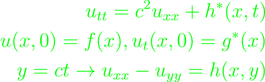
By choosing starting conditions and integration, the general solution in terms of the original variables is

There is a method to aid in solving the integral. In general, the functions in question are the linear hyperbolic equation L[u].

L here is taken to be an operator, and the coefficients to be differentiable functions over (x, y). We can find the adjoint operator to L through construction.

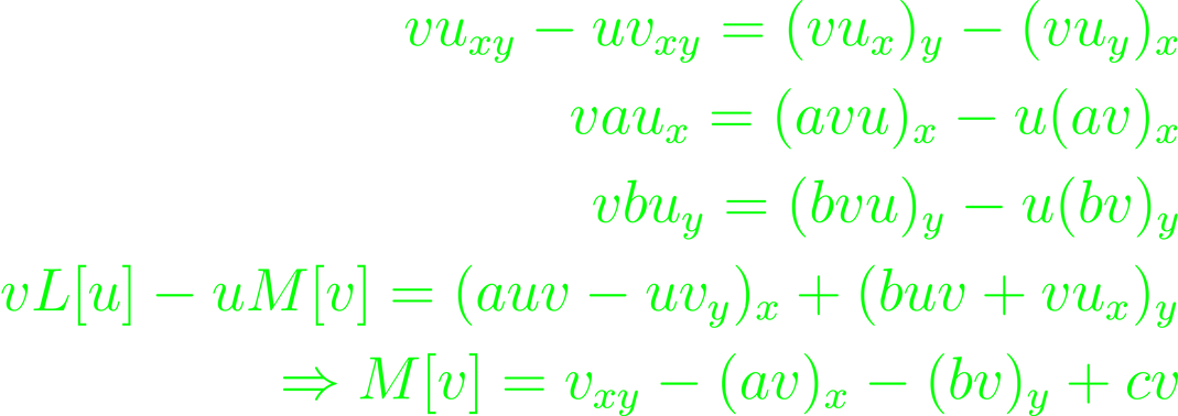
Integration and application of Green's theorem will enable a solution along a smooth initial curve. The computation is not necessarily difficult, but not very interesting. Instead, let's take a look at the solution as we limit the contours of the curve. Choosing two points on the curve and the point in which the axis-perpendiculars of the points intersect form a contour with the initial curve, bounding some area D. For a part of the curve, this can be done repeatedly, giving a series of bounded areas that enclose smaller ones constructed in the same way. The area associated with the external point's y-component is the graphical representation of the curve's characteristic. For parabolas for example, the y-component has two intersections with the initial curve, so the characteristic is not unique and the Cauchy-problem is not solvable.

The solution of a linear hyperbolic equation with prescribed conditions on a characteristic and monotonic increasing curve, is then a kind of equation that is not solvable through the Cauchy problem. It's a specific problem, but it has a solution. The Goursat Problem can identify the monotonic curve in the first quadrant by iteration.

Fourier Series & Separation of Variables

We should already be familiar with fourier series as a concept and how to apply it to functions. They have a lot of uses in applications from physics, information theory and anything that otherwise deals a lot with integrals. That is for their ability to make "problematic" functions integrable. Piecewise smooth functions can, for example, always be evaluated piecewise. That can be bothersome, if not for some shortcuts that one might find. Of course, the chief of these is the possible periodicity of the function. Periodicity and smoothness are independent.

The Fourier Series itself is a series of transformations achieved through an integral, so it can only ever be applied to fully piecewise integrable functions. The Fourier series uses the periodicity of the trigonometric functions to approximate it. For now we take the interval to be 2π, but departing from that is a trivial coordinate transformation x → lt/π where t is the new variable and l is the new interval. Nominally, we can write such a function as

We generally want the Fourier series to converge towards some defined function, but convergence is a varied term. The Fourier Series can either converge pointwise, uniformly or mean-squarely. Pointwise convergence is the easiest construction and the weakest of the three. It asks that |f(x) - s(n, x)| → 0 as n tends to infinity. Uniform convergence is the next stronger definition of convergence, using the maximal norm. It requires that max|f(x) - s(n, x)| → 0, n → ∞ and usually x is constrained between some a and b. One can make this a global property by setting a ≤ x ≤ b with a → - ∞, b → ∞. The mean-square convergence has functions converge in the space of square-integrable functions. The norm in that space introduces an integral, so that will show up in the convergence definition.

All these are basics when handling the Fourier series, but in actual application, one finds oneself moving in complex domains often. There are exponential forms of the Fourier series that can be identified through Euler identities of trigonometric functions. It lets us rewrite the Fourier series as follows:

As the Fourier series depends heavily on the integrability of the function, there is an obvious interest in expanding integrability outwards from the Riemann definition. This is of course the Lebesgue integral for expanded integrability, and integrability on non-trivial manifolds. Functions that are Lebgesgue-integrable can of course also be subject to Fourier representation. It allows for integration of non-globally continuous functions without thinking too much about the repercussions of those inconsistencies. Take a piecewise continuous function g(x) on some closed interval [a, b]. Then, we can say that

This can be applied to all discrete continuous intervals of g(x). If we now take g(x) to be smooth and periodic (with 2π) as well, then the Fourier series s(x) = 1/2[g(x+) + g(x-)]. A continuous function with periodicity 2l and piecewise continuous derivative in the interval [-l, l] and f(-l) = f(l) has a uniformly and absolutely convergent Fourier expansion. The basis of this uses trigonometric functions, so the periodicity is 2π. Again though, a transformation can give this universality. The same goes for piecewise smooth functions in [-l, l] with periodicity in 2l, which have uniformly convergent Fourier series in all closed intervals without discontinuity. By the Gibbs phenomenon the behavior of each partial sums of the Fourier series can't approach the function uniformly over any interval containing points of discontinuity. These are the basis of integrability of Fourier series and the existence of Fourier series of the derivative. If f is piecewise smooth in every finite interval and absolutely integrable on R, then

This is based in the Fourier integral representation

Separation of variables is somewhat of a physicsist's favourite tool for solving differential equations because it's easy and intuitive, but the way they tend to use it is usually kind of wrong - or at least imprecise. Obviously casually dividing by a differential can be problematic, so why does it work in some cases? This method will make sense to apply at second order or higher, and we begin with the homogenous case. Homogenous equation can always be written in a canonical form dependent on u(x, y) and it's homogenous derivatives up to arbitrary order (we will examine second order first, so that's the order we'll use here). Parabolic equations have no second order derivative contributions, if they are opposite, the equation is hyperbolic and if they are identical, they are elliptic. Trivially, the viability of the method depends on the separability requirement of the variable function u(x, y) = X(x)Y(y). Dividing out X and Y then makes it possible to separate the x-terms and y-terms on opposite sides of the equation. Then, derivatives of both sides of either variable have to evaluate to null. We consider what stands on either side the /separation constant/ \lambda, defined up to a sign. We can use it to actually separate each equation, substituting either side with \lambda. This is where we can multiply X (or Y) back in to get a prettier form of the differential equation. This nets us two homogenous differential equations of first order, connected by the separation constant.

Eigenvalue Problem & Special Functions

There is a method to further generalize the separation of variables, through Sturm-Liouville. Along the way we'll disambiguate some of the linear algebra we should in principle be already acquainted with. I'll not draw parallels between the two here, because it occurs across a lot of area, and things like these are really best saved for the Concept Deep Dives. Separability safely transfers a valid differential equation into a convenient form, and we introduce some convenient short form definitions to get to the Sturm-Liouville equation (SLE) which induces a self-adjoint operator (we assume that n ≤ x ≤ m).

The SLE is regular, if for Ay(n) + By'(n) = 0 and Cy(m) + Dy(m) = 0, the constants are real, nonzero numbers. λ needs to be set, and if the resulting system has a nontrivial solution, it's an eigenvalue with the induced solutions the eigenfunctions.

The SLE can also be periodic, if there is an n and m as prescribed, so that p(n) = p(m), along with y(n) = y(m), y'(n) = y'(m). This case can be checked either through example, or disproven by checking that λ < 0. It's also notable that λ = 0 here implies a trivial eigenfunction 1. For any y, z of the operator L's domain D(L) the Lagrange identity can be written directly

An eigenvalue can occur more than once for a SLE. This marks the multiplicity, and while the eigenvalue is set as many times in the system as its multiplicity, it will have several different eigenfunctions, which are all linearly independent. Linear independence of functions is really the same as orthogonality, which takes the regular definition of their outer product vanishing. We keep in mind the definition of that product.

with a weight function ρ > 0. Let's keep this definition in mind, so we can make a few explicit statements about the SLE. We could take the coefficient functions p, q, s to be continuous in [n, m] and the eigenfunctions of λ, ρ continuously differentiable, then through explicit computation, they turn out orthogonal to s in that interval. This is automatically true for all eigenfunctions in a periodic SLE.

For a regular SLE with s > 0 only has real eigenvalues due to the definition of L = -λ. For two solutions f, g of the SLE, then we can retrieve the definition of the Wronski determinant through Abel's formula: p(x) W(x; f, g) = α = constant. Together, the eigenfunction of a SLE unique up to some constant scaling factor. If the SLE is regular and self-adjoint, the sequence of real eigenvalues is strictly ordered, with multiplicity one, and infinite. There is no upper limit for this sequence.

For functions of the square integrable space the Schwarz inequality holds in general. From that, constructed functions with pairwise orthogonal square integrable functions with a weight function ρ

For regular SLEs, the eigenfunctions are complete in the space of piecewise continuous functions on some interval [a, b] with respect to some weight function ρ(x), any piecewise smooth function on [a, b] satisfying the boundary conditions of the SLE, is expandable into a uniformly convergent series with coefficients

A SLE is singular when given on a (semi-)infinite interval, when either coefficient p(x) or s(x) vanish, or either become infinite at at least one end of a finite interval. The system requires appropriate linear homogenous boundary conditions. Occasionally, boundedness of y(x) at singular end points needs to be prescribed for the integral to remain computable. For appropriate y(x) and z(x), and

A singular SLE is self-adjoint. Square integrable eigenfunctions correspond to distinct eigenvalues of a singular SLE are pairwise orthogonal with respect to the weight function.

Boundary value problems consist of a function induced by a linear operator of some order n and n many boundary operators, which are polynomials evaluated at the borders. Assume continuous coefficients p(x), q(x) and a function f(x) on [a, b], then the boundary value problem L[y] = f, U[y] = A, V[y] = B will have a unique solution for any given constants A, B or else there is a nontrivial solution for L[y] = 0, U[y] = 0, V[y] = 0.

If we take L[y] = -f(x) in [a, b] with

where each y is linearly independent. Through variation of parameters, the constants A, B will be replaced by arbitrary functions of x, which are defined by

Introducing the Wronski-Determinant W(x) gives expressions for the u functions and with that a solution to the system

which takes the form of a Green's function.

Boundary-Value Problems

Generalizing the initial boundary-value problem extends the boundary condition onto the entire length of the function. The problem is still independent of time, as the boundaries better not move. The boundary-value problems are associated with elliptical differential equations. Such differential equations of second order has the general form

The simplest of these problems is the Dirichlet Problem: u = f(s) on a piecewise smooth curve. Let the harmonic function u(x, y) in a bounded domain D be continuous in D ∪ B where B is the boundary of D. The maximum of u on D ∪ B is trivially in D (inclusive) or B. If it's not in B, then the harmonic nature of u forbids a global maximum. Similarly, the minimum too exists on the boundary B of D through substitution of u -> -u.

The solution to a Dirichlet problem is unique through the boundedness of D as well, since the solution is directly dependent on the associating with functions on the boundary. By the Maximum/Minimum principle, identical functions on B become identical for the interior of D as well. They are also (intuitively) continuous.

Assume a sequence of harmonic functions in D, which are continuous in D ∪ B, where B is the boundary of D. If it converges uniformly on B, then its values also converge uniformly on B. Through continuity, the sequence then also converges uniformly on D ∪ B.

In higher dimensions, boundary-value problems can be used to model 3-dimensional wave/heat equations. This obviously calls for a wave equation in 3-dimensional space

Similarly, the heat equation has a set form for which we just insert the ∇ operator instead of the derivative.

Solving the wave equation in 3 dimensions is an almost thoughtless process for physics students, on account of spending several semesters doing exactly that. There is however a non-analytic approach that comes more from linear algebra. This approach is a little more abstract, and possibly more work in application, but not uninteresting. For the sake of this, begin with the nonhomogeneous initial boundary-value problem

in a domain D bounded by B. Given two initial conditions f and g, with ρ a real, positive continuous function and G a real, continuous function. This gives the homogeneous problem

Assume the boundary conditions to be such that only the trivial solution solves it. Any solution of the nonhomogeneous case will have to be of the form

where φ is a function satisfying the boundary conditions f and g. To do an example of wave functions on non-trivial geometry, imagine a rectangular membrane (a * b) which is excited into vibrations.

The next step is finding the eigenvalues and eigenfunctions to construct an expression of φ to insert into the definition of u in elliptical problems.

Take the specific solutions from the initial conditions. Roughly the same method solves the time-dependent boundary-value problem.

The operator form of the boundary-value problem should seem familiar to those who have read the Concept Deep Dive about the Green's function, and that also means that technically there is a solution to the system that is a Green's function. At the same time, there's some extra features to the problem that reveal themselves through the properties of the boundary-value problem, which lead to different methods of solving the associated Green's function. We recapitulate that as a solution, the Green's function will show up as follows

with n the outward facing normal vector on B. The corresponding Green's function has to satisfy a few conditions, that we know to be true by that form alone.

and the continuity in its variables. The derivation with respect to n however has to be discontinuous at (ξ, η). To actually find this Green's function, it can be convenient to split it into the Free-space Green's function F, which satisfies the first constraint, and add a function g to it, which will balance it out everywhere else. Stepwise identification of these parts is the Method of Green's Functions.

Integral Transform Methods

Using the Green's function as a jumping-off point for solving a complicated function will kinda suck, because applying the method for Green's functions presupposes that the user is good enough at solving integrals to construct both the integral, and hence the operator that'll be applied to the Green's function. On the bright side, there are a bunch of ways to approximate a complicated function with a bunch of really easy functions using linear superposition. However, some of these methods will require some basic understanding of the common integral transformations.

I'll assume knowledge of Fourier transforms, and won't lose too many words about it, but it's of course the most well known and probably most widely used (at least knowingly, we will ignore the Legendre transformation popping up everywhere for now) of the bunch, and can't really be avoided here. Some of the properties we'll name, and later exploit for better access for solutions. Some functions are invariant to Fourier transformation (we call these self-reciprocal rather than invariant in this context). We'll note for praxis points that these approach a Gaussian distribution curve, with the function approaching 0 at both inifinities. Reciprocality is based in the cyclical nature of the transformation, wherein repeated application on the same function will return to the same function after 2 iterations. The Fourier-transform as an operator then is the inverse transform to itself. By definition, the linearity and scale-invariance of the transform is trivial. From this scale invariance, shifting the variable will generate an exponential factor with the shifting constant in the exponent. Explicitly, this can be verified by coordinate transformation to counteract the shift constant. Differentiation of a Fourier transform generates a factor of ik, which will repeat for every tacked-on differentiation.

There is a different transformation that interacts very comfortably with the Fourier transform, namely the Convolution. It's defined as follows

It's commutative, associative and distributive. More interestingly, the Fourier-transform of a convolution will output the product of both respective Fourier transforms. This can easily turn into Parseval's formula through choosing one of the convoluting functions to be the complex conjugate of the other.

In the case that an integral turns out so ugly that it's not exactly solvable through mortal means, then there's always the physicist/engineer's favourite method: The Approximation. But how does one approximate an integral?

An integral should first and foremost output a function, and approximating those is always a question of the asymptotic. Remember, that every time we attempt such a thing, a limit is involved, in which we push something (usually an order of terms) towards infinity. Because a lot of the functions that become problematic are problematic because of some exponential term that refuses to cooperate with ones efforts, let's generalize the problem as

θ is what's known as a phase function. By construction, we should want to know the asymptotic behavior for x and t. It might also be interesting to look at the limit of t to infinity, while x/t remains fixed. In general, with t → ∞, the phase rotates very rapidly, i.e. the integrand oscillates very quickly. Because it oscillates around the x-axis, neighboring contributions will cancel each other out. The exceptions to this are stationary points of the phase. These are best found through a derivative, but since the integrand is of a somewhat inopportune form for that, we'll have to settle with the Taylor series at that point. To make it easy, it suffices to replace both F and θ with their Taylor series. Evaluating that will give a decent estimate for the solution.

A different common transform is the Laplace Transform.

It exists for piecewise continuous intervals [0, X]. It's linear and scaling the variable to f(cx) will yield a transformed function of

and a shift of

The Laplace transform of a differentiated function will give sL[f(t)] - f(0). The integral comes out as expected from this observation. The convolution interacts with the Laplace transform the same way it does with the Fourier transform.

Nonlinear Partial Differential Equations with Applications

The expectation that things be linear is one I've only ever seen in school or from economists, neither is the level any self-respecting STEM enthusiast should shoot for. And now that I've gotten my daily quota of picking on economists done, let's abandon the requirement of linearity now and take a look at our favourite differential equation: the wave equation.

Linearity, is really the condition that f(ax + x') = af(x) + f(x') for some constant a. The simplest way to not make this linear is to make a not a constant anymore. The general form of a non-linear one-dimensional wave equation is

We should notice a few things before trying for a solution, because the non-linearity will disqualify a number of the methods that were used for the linear case. Linearity also eliminates degrees of freedom, so losing that will make significantly fewer ones solvable. Having the coefficients not being constant or dependent on the variable, rather than the value of the function, will remove superposition as an approach to solve the equation. It can also hide terms that will nudge the equation between types. Solving this equation is not technically a new approach in concept, but the methods will be slightly different, so like always the first relevant differential is

We remember this to be generally true for all u(x, t), and by the general method of solution, the equation is expected to resolve geometrically on some points on a characteristic curve Γ where dx/dt is the slope of Γ. The function u is expected to be constant in time for wave equations (which is also visible in the general form of the wave equation), so there emerges an explicit expression for a(u), namely dx/dt. The characteristic curves, that up to this point were mainly a nice geometric concept, will now become the main method of solution.

For the constancy of u with respect to time implies constancy along its characteristic curve, which in turn will fix the coefficient a(u) as well. The set of characteristic curves will then resolve into a set of straight lines, where the slope is fixed on a. This leaves one degree of freedom for the problem, which is directly fixed by u. The full characteristic form of Γ gives in itself a system of equations:

Setting u = f(ξ) will fix Γ and by setting

With this the slope of the characteristic curve has become non-constant with respect to ξ. The results can be verified through differentiation, which is not difficult in this general notation.

Since the slopes of the characteristic equations need no longer be identical across all solutions, there will be systems, in which the characteristic curves intersect at finite, but large enough times. These are, for examples, dispersive waves. Take some polynomial of derivatives P and plane wave solution u, then the linear partial differential equation Pu = 0 can be solved given a relation P(-iw, ik, il, im) = 0, where each of the arguments substitutes one coordinate derivative operator. This is the generalized dispersion relation. Much of the following discussion is already covered in the series on General Relativity, though of course that is a rather specific example. Seeing as the approach is one to one though, I don't particularly care to repeat it here. The same goes for the nonlinear case. I'll give the general form of the equation, and we'll leave it at that.

As applied in GR, some non-linearity can be neglected, if the wave amplitude is small enough. Assume however, that the amplitude be finite, but large enough so that higher order terms can't be neglected. For finite waves, Stokes theory is the go-to approach, since it considers the boundary conditions. With a frequency of ω, the Stokes expansion is as follows

This is the nonlinear dispersion relation. The linear case can be recovered for a → 0. Resolving this through the Whitham equation, as in the case of the dispersive waves will yield a coupled system of the form

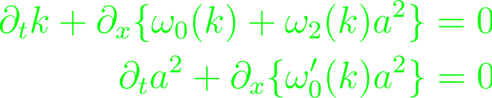
which after expansion can be written in a matrix form and transferred into a determinant equation.

The term in the square root will decide over the reality (hyperbolic character) of the system. The imaginary case is analogous to an elliptic system. These are unstable for t → ∞, and in many cases it's valid to dismiss these solutions as unphysical.

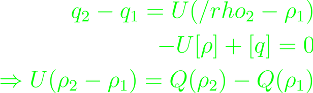
A special kind of non-linearity is discontinuity. Such can be found in shock wave scenarios, for example. One access to the system is through the conservation equation for waves, which in itself shouldn't change. Assuming q = Q(ρ), the equation resolves

Deconstructing the integral will give a condition for the integrand to vanish, which in turn gives the shock condition

At points of continuity, the conservation equation holds, and at points of discontinuity the shock condition does. For large differentials,

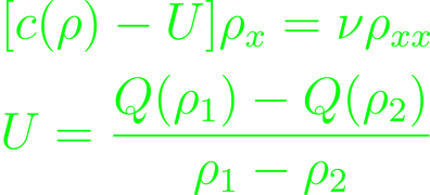
where the second and third terms describe the effects of nonlinearity and diffusion respectively. The simplest cases are of course c being a constant or vanishing. The solutions each turn out in form of a plane wave solution, though of course the non-vanishing case is not a trivial one. With the help of the linear equation we can recover the dispersion relation

This is a diffusive wave, decaying exponentially over time. The vanishing case will reduce to a linear diffusion equation. The constant U will have to be determined and decides whether the solution diffuses further or not. It can be determined through applying integration to

This construction is closely related to Burger's equation and its solution, which should also have received a treatment in the GR section. It's mostly busywork and integrals, but it's also not unimportant, so maybe this is a perspective topic for a future deep dive.