Aerodynamics
Aerodynamics: Introductory Concepts
It's confounded me that fluid dynamics weren't really taught stringently in any of the courses I had to take. And then occasionally some fields of physics borrow concepts from fluid dynamics, which always irritate me, seeing as reading up on fluid dynamics isn't exactly an intuitively easy process. The book I'll be working off is the Fundamentals of Aerodynamics which is a bit chunky, but will hopefully be a good substitute for the actual course.
Though the title focuses on aerodynamics, it contains a good amount of more generalized fluid dynamics to get there. For information on gas dynamics and hydrodynamics I'll postpone for another time. Since the book is a chunky 1100 pages, I'm fully expecting to interrupt it for longer time-spans, so I can insert a few other segments, and take a break. After all, aerodynamics is an applied science, meaning I'm expecting the experimental approach, which is not exactly an approach that is easy on my brain. I'm still choosing to do this over theoretical fluid dynamics, because this will serve as a combination of a lot of interesting concepts in classical physics, and maybe lets me think a little differently about airplanes, which I happen to think are very fun anyways - probably in the same way other people like cars.
The book introduces a few variables that the reader will have to get used to, so I'll take them as they come. It's probably not much of a surprise that a lot of aerodynamics borrows concepts from thermodynamics. That means that we'll work with the usual quantities present in the ideal gas law, i.e. pressure, density and temperature. Because the flow of air will play a role, the flow velocity will be interesting to pick up as well. Their definitions can be taken exactly as they show up in thermodynamics - it's classical physics, everything has one definition here, and that makes things very comfortable to think about.
Let dA some infinitesimal area at point B, dF the (net) force exerted on dA through some pressure, dv an infinitesimal volume element around B, and dm the mass of the fluid within dv, then the pressure p and density ρ are defined:

I'll hold off on the temperature, because its definition is somewhat dependent on a small number of other factors, and even though the book provides a formula for a case, I'd rather set the regime first and explain why it's applicable, before committing to an expression. Flows are qualified by sort of collective motion of particles. It's not usually much good to look too closely at what the individual particle within a flow does, but to quantify what actually happens in the flow, it is split into volume elements, or rather fluid elements, which are the objects that can receive attributes like velocity. The flow velocity then isn't as much a vector as it is for solid objects, but rather a vector field made out of "streamlines". They experience a variety of forces, notably friction. As the fluid elements are treated as objects in space, the streamlines can exert fricition on one another and thus exert force tangentially onto the streamline. This is called shear stress and is defined like the pressure, though using the tangential force rather than the perpendicular one. Each fluid will have an empirical viscosity coefficient, which allows to shear stress to be defined with respect to the velocity gradient.

Shear stress and pressure will create a distribution that will describe the entirety of external forces acting on a body within aerodynamics. Because one acts perpendicularly and the other tangentially to the surface of the object in question, they will always be locally independent of one another. They are also both defined by essentially velocities, a quantity that is subject to relativity, so the actual property that becomes interesting for the forces' definition are relative velocities. The flow velocity far ahead of the object is the relative wind, the one far away from the object is the freestream. The definitions of lift, drag, and angle of attack stem from the geometry of an object in a stream. The lift is the perpendicular component of aerodynamic force (with respect to the freestream velocity) and the drag is the complementary parallel component. The same definitions can be done with respect to the chord (the linear distance between leading and trailing edge of the object) to get the normal force and the axial force respectively. The angle of attack is that between the lift and normal force (or between the drag and axial force). Because of the geometry of the problem, the forces are usually considered first per unit span. What follows is "just" scaling the numbers up and plugging it into the integral. Logically, all quantities defined previously are intuitively functions of the effective area, i.e. are defined mainly by the geometry of the problem. Some will combine together into coefficients.

It's convention to mark the coefficients in 3 dimensions as capital letters and the ones in 2 dimensions as lowercase ones.
The normal and axial forces on a body, trivially, are functions of distributed loads of pressure and shear stress. They will also generate a moment on the leading edge of the body. Classical physics likes to boil these down to forces acting on a point, but doing so isn't exactly easy in aerodynamics. Where often we are interested in finding the center of mass in classical mechanics, the idea becomes to find the center of pressure, i.e. the point that if all pressure arrows were to not encounter any resistance, the object would fold into. Mathematically, this would mean that the integrated effect of the force distributions are zero at that point. For the dynamics, this point is where the resultant force will "act upon".
The differences between the motion attached to the center of pressure and anywhere else isn't the resulting velocity, but rather the resulting rotation. If a force is attached to the center of pressure, it should not generate any rotation, but everywhere else, it would. Each distribution of force, i.e. each set of flows will generate its own center of pressure.
It's probably apparent at this point that completing aerodynamic flow computations isn't always an easy task. As a consequence, it would pay off hugely to identify similarities in flows. Definitionally, flows are similar, if the streamline patterns have similar geometry, the normalized distributions of velocity, pressure and so on are the same when plotted against non-dimensional coordinates, and if the force coefficients are the same.
These criteria are of course also dictated by the geometry of the bodies involved in the problem. The flows then are dynamically similar, if all solid components of the problem are similar, and the similarity parameters are the same. In the case of aerodynamics, said similarity parameters are overwhelmingly set by the Reynolds number and Mach number. Both can be derived through the Buckingham-Pi Theory, taken from dimensional analysis.
Before taking a closer look at the different forms of flow, there is a fluid dynamics scenario that is easier, and introduces the concepts for the more complicated problems. This is the buoyancy force in fluid statistics. Objects immersed in static fluids will still experience forces even without relative motion between the two. Each fluid element experiences both pressure forces from surrounding fluid being exerted onto its own surface, and gravity pulling it down, usually along the z-axis. The net pressure force can be determined by subtracting the pressure on the top surface and that on the bottom surface. If the fluid is static, pressure forces to the sides cancel out to 0 and can be ignored. The net pressure force turns out -dp/dy. For the object itself to become stationary, the sum of net pressure and gravity must be equal. This leads to the hydrostatic equation

Take a rectangular body of width and length l and height h, and submerse it in some fluid. The vertical force on the body due to pressure is noted as F. The difference of pressures can be obtained through integrating of the hydrostatic equation.

The weight of the displaced fluid will then be equal to the bouyancy force acting on the body. This statement is the Archimedes Principle which is often found attached to the anecdote in which said Archimedes is tasked to determine the material of a crown.
Flows can be organized along several parameters: Continuity, Viscosity, Compressibility, and their Mach number, the last of which will land the flow in a subsonic, sonic or supersonic regime, which the reader will presumably be familiar with. We'll check each of them in turn.
All fluids are, in essence movement of an ensemble of particles. This carries a certain amount of random collisions between the particles with it. A flow can then be classified by the frequency of collisions or rather the (mean) distance traveled between collisions. This is considered the mean-free path \lambda. For mean-free paths that are orders of magnitudes smaller than the particle itself, the surface of the flow can be considered continuous, making it a continuum flow which is contrasted against flows for which that is not the case. This would make it a free molecular flow.
Viscosity is marked primarily by the transport phenomenon of the flow. It will involve friction and thermal conduction, i.e. phenomena in which the bodies within the flow can have their properties changed. Flows for which that is not the case are considered inviscid. Of course this is an odd requirement, and according to expectation, mathematically, inviscid flows are those for which the Reynolds number approaches infinity. In practice, a very high Reynolds number can be considered inviscid already.
The flow's density can be constant, which will mark it as incompressible. This, too, is an odd property, so the mathematical description will also involve a limit. In this case, this will be a low Mach-number. For practical reasons, this will be a Mach-number below 0.3
Viscosity mainly affects the area of the flow that is close to the body. These are the boundary layers, essentially thin layers of the flow, in which the dissipative effects happen, meaning they are worth looking at separately. The force that the boundary layers exert on the body will come together for the common (not quite accurate) explanation of how the wings on an airplane work. On the molecular scale, particles in the boundary layer stick to the surface of the object, meaning they have zero relative velocity. Classical mechanics dictate that the force it exerts directly onto the body's surface is going to be great enough to create a higher friction than the force that is exerted by the flow on the particles.
When thinking about aerodynamics, I think even the layman will imagine the prototypical airflow diagrams with a wing, or a car in the focus. The lines in these diagrams are the pathlines or streamlines. As discussed, a flow is actually an series of elements traveling through space. The path traveled by some element then defines the pathline. Elements can pass through the same point in space, but take a different path. In this case, the flow would be considered unsteady. As discussed, the streamlines are pathlines that tangent the surface of the object. It too can differ over time in unsteady flows. Unsteady flows are (if I'm not mistaken, the book does not specify) more at home in the field of chaos theory. A pathline picture would include all the possible paths of the flow over time, while a streamline picture has more of a snapshot nature. In a steady flow then, the pathline picture and the streamline picture are the same. These lines are all curves in space (three dimensional space), so it can be parametrized as a 3 x 3 matrix. This is best done through the vector field and the parallel directed element of the streamline.

Now that the motion of each element in the flow is fixed on coordinates, it should be noted that such elements are very much subject to change. This is of course because it might interact with other fluid elements and a motion in three dimensional space will have the additional rotational degrees of freedom. How much the element is rotated and distorted is chiefly dependent on the velocity field. Traditionally, problems like these will be solved by application of the curl operator and the angular velocity ω. Twice the angular velocity will define the vorticity ξ = 2ω = ∇ ⨉ V. If the vorticity is 0 at every point, the flow is irrotational, meaning that no all fluid elements have no angular velocity. Their motion consists only of translation. Otherwise the flow is rotational. Through the rotation it's pretty clear that the angle of certain edges of the elements are subject to change, but what adds distortion to the process is the fact that the volume is a constant over time. In two dimensions, this limits the distortion to parallelograms. Over time, in a rotational flow, a two dimensional element will require an additional parameter, meaning the angle in between two adjacent edges of the element. The strain then is the change of that angle. Convention is to describe a decreasing skew angle as positive strain.
Often it's convenient to view the stream as a function of spatial coordinates. For stable flows, this is not only formally correct, but also very useful. Such a function is defined as the stream function Ψ. Each streamline is given by a setting a constant stream function. The difference between the values of the stream function at two different points should be equal to the mass flow between the streamlines that the coordinate characterizes. The geometry of the flow field will dictate how exactly this difference turns out. In steady flows, the mass flow along one streamline could be views as if mass transport in a tube around that streamline. This mass flow should be constant along the tube to avoid turbulence. This justifies the stream function being composed of constants. Naturally, for this to make sense, the stream function should be continuous, so it should have a derivative. To define it, one can use the mass flow definition to construct the basic definition for derivatives. Taking δ n to be the difference between two streamlines.

From the generalized geometry, the mass flow develops

Depending on the dimension of the problem, a set of differential equations emerge. As the velocity is presented as a field, and physically, the flow must be agitated in a way previous. The type of field is somewhat reminiscent of electrical fields. This implies something like a velocity potential, or at least a treatment of the maths that will treat the velocity like the consequence of some potential. In that way, the ideal of the velocity can be directly mathematically linked with the stream function.
Inviscid, Incompressible Flow
Before getting into the meat of actual "applied" aerodynamics, a short reminder of Bernoulli's equation might be in order, as it will be a key tool for analysis. It's contrasted against Laplace's equation in it's use in inviscid incompressible flows. Bernoulli's equation was determined to give the relationship between pressure and velocity in such a flow, spelling

When the body forces are removed from the system, the equation can be depicted easily in the form of a differential equation. Solving it will yield Euler's Equation.

It's solved using by applying an integral to both sides This will add the constant and recover Bernoulli's equation. This constant will be an indicator of the body forces. Other than an object in a flow, there are other ways to alter the aerodynamic model. Often, the flow is constrained in space, for example by the walls of a room. The simplest of these constraints would be that of a "wind tunnel", meaning a duct with variable cross section. In usual application, it's often assumed that the variation of the cross section is low, and so the flow is considered uniform along all axes but the length of the duct (let's consider this the x-axis for short). This will make the problem effectively one-dimensional, and while this is technically only an approximation of a three-dimensional flow, the approach produces results that are good enough for applications. Not dissimilar to the treatment of vector fields in electrodynamics, the continuity equation should hold.

where the first term describes the perturbations in the field. For a steady flow, it disappears. The integral then splits into the three constraints on each side, and the upper/lower walls of the duct. The flow should be perpendicular to the wall, so that integral too, should disappear, meaning that only the entrance and exit of the duct (convergent and divergent duct) actual contribute to the result.

For constant flows, the densities are static, and so are equal. They can be canceled in the final equation. A particular type of funnel with a minimal cross section at the "throat" and diverging walls to both sides is a venturi. From Bernoulli's equation, the velocity of the flow increases as the walls of the duct converge, so they are at their highest at the throat of the venturi. To both sides of the throat, a pressure difference is built up. It can be used to transport material against the gravitational force.
A similar concept of pressure difference is used in pitot-tubes to measure airspeeds. They are still in use on modern airplanes today. A pitot-tube is a small tube angled at 90 degrees and leading into a pressure gage. The incoming flow has some pressure p and velocity v. The random motion of the particles in the flow also exerts some static pressure. Considering a wall with a small hole leading into it at a perpendicular angle. The plane of the hole is parallel to the flow, since the flow moves over the opening. The pressure at the hole (and down until it ends) then is only the static pressure.
Usually, the pitot-tube is held into the flow, so that the open end faces directly into it. The flow will transport its fluid into the tube, until the tube is full (the pressure gage is a closed component). Once the fluid has filled the tube, it stagnates and its velocity drops to zero. It effectively closes the tube for the purposes of the flow. The pressure at the stagnation points, which includes the pressure gage is the total pressure. The difference between static and total pressure allows the calculation of the flow velocity using Bernoulli's equation.

For the future, the pressure coefficient can be defined to introduce a dimensionless pressure.

Incompressibility comes with a few perks. It's been mentioned that ρ = 0 for incompressible flows. This however means that the fluid element of fixed mass moving through the flow field has a constant volume. In math, this quantity is described by ∇ V, meaning that the divergence of velocity is zero for incompressible flows. This result can also be derived from the continuity equation

We can reintroduce the generating potential for the flow velocity to apply it directly to the statement above, then reintroduce the stream function to get a differential equation

For applications, boundary conditions are defined by the geometry of the problem. This will either be a infinity boundary condition, or some wall boundary condition. The former is the easier of the two, because no geometry takes place. At infinity, there just needs to be some flow velocity defined.
The wall condition uses a unit vector n normal to the surface interpreted as the wall, and the distance along the body surface s

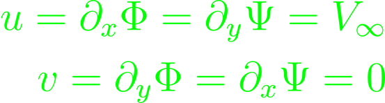
Uniformity of flow implies first incompressibility and irrotationality. The velocity potential then takes the form of V = ∇ Φ. Following a similar logic yields

The two components of Φ are independent in their variables. The consideration for the incompressible stream function is basically the same. The circulation in a uniform flow is given by

A flow can of course have a source from which it emerges. Take the flow emerging from a funnel at a large limit, for example. For this, the considerations above are basically identical, though of course it makes sense to adapt polar coordinates for the field. It becomes more interesting when inspecting a doublet flow, a degenerate case of a source-sink pair which creates a singularity in the potential.
It begins with a source of strength Λ, and a sink of equal and opposite strength, with some distance l between them. At any point in the flow between them:

Of course this is meant to be a closed system, and best viewed in polar coordinates. Trigonometry should easily give

in the limits. In analogue:

κ here is the strength of the doublet lΛ. As such, the problem can be viewed as discrete doublets of strength κ at the origin, with the flow lines moving opposite one another. This, superpositioned with a uniform flow, will simulate the flow over a circular cylinder. In true wave-function fashion summing over the flow functions will yield the accurate new flow function. The pressure coefficient

Meaning that the pressure varies somewhere between 1 and -3. The squared sine-wave can be mapped over the surface of the cylinder, so that it's symmetric over the axis running along the chord.
A flow without source, but where all streamlines are concentric circles with the same orientation around a shared center point is called a vortex flow. The speed component of the flow-field at any point is zero in radial direction, and something with an inverse dependency in r in axial direction. It can be constructed to be physically incompressible, and except for the origin, one can treat the rotation to be zero. To get the exact axial velocity component, take the circulation with some radius r

Combining the vortex flow with a non-lifting flow over a cylinder adds a vertical direction to the nonlifting flow, introducing a lifting component. Practically this could be achieved by placing a rapidly spinning cylinder into a non-lifting flow of a wind-tunnel. This is very similar to the effect by which a spinning ball can curve in the air. The superimposed flow function and velocity functions come out as

Any potential naturally tends towards zero, so solving the system for the coordinates at which both functions come to zero will determine in which direction the cylinder is pushed by the combined flows, as long as the stagnation point falls outside of the body. For the method of determining the generated lift, there is a relatively simple theorem. The Kutta-Joukowski theorem states that lift per unit span on a manifold (read, 2-dimensional body) is directly proportional to the circulation around the body. This is a good way to find the generated lift on simple geometries - though the modern approach is a little less pretty, and thus, inherently a bit less interesting to me. Still, it'd be wrong to not include it in a treatment of aerodynamics, so here goes.
The Source Panel Method is a numerical method to solve for the flow over an arbitrary body given the singularities and a uniform stream. The body can be approximated by tracing its outlines with infinite, infinitesimal single line sources. By also dividing the distinct manifolds of the object's surface into small sheets ds with the strength dλ, the infinitesimal potential can be derived, and with that, an expression for the full potential can be solved for using methods for analyzing differential equations.

This reduces the problem to finding appropriate source sheets to construct the problem with. This is where the method becomes numerical. The object can be constructed by lining up infinitesimal panels with indeterminate strengths, each of which will come with its own boundary condition, defined so that the mid-point of the panel (also called the "control point") experiences zero flow velocity. This is because in the usual consideration of the problem we imagine the shape itself to be static and the source panels aren't fixed to one another in any different way.
For each point P in the flow with an indexed distance to any point on the j-th panel (sorted arbitrarily, but practically in order of distances), the velocity potential is as discussed. The distance then needs to be parameterized in a way that makes sense, usually in polar coordinates. To retrieve the pressure coefficient at a control point, its velocity potential needs to be found by applying what's basically standard mechanics to each of the panels, while taking the relative slope to the chosen point into account.
Incompressible Flow over Airfoils
The really interesting objects in aerodynamics are things that are supposed to fly. Obviously a lot of engineering has gone into this, so that it flies as intended. Airfoils are the famous shapes of airplane wings. In addition to the cord line that gets sketched through the length of the foil, one can introduce the "mean camber line", a line that's usually above the chord line, splitting the difference between the the upper edge of the foil and the chord line. The "camber" is the area between the mean camber line and the upper edge. If it is above the chord line, it's considered positive, if it's below, then negative. When we refer to the thickness of the foil, we mean the maximal distance between upper and lower edge, perpendicular to the chord line. Usually, the rounded edge of the airfoil is the leading one. This is the case we'll discuss unless stated otherwise.
The airfoil has a characteristic angle at which lift generation is maximal. Beyond that, the leading edge of the airfoil is pushed upwards and part of the flow will separate off into a turbulent portion. This is the condition under which the plane will stall. Positive cambers will usually have a negative zero-lift angle of attack, and symmetric airfoils will have one of zero.
The shape of the airfoil is such, that the flow over the trailing edge can be smooth, depending of the angle of attack. To identify, when exactly this is the case, there is the "Kutta Condition", stating that a solution for the circulation exist for any foil and angle of attack for the flow to come off smooth at the trailing edge, i.e. this solution exists. If the trailing edge is angle is finite, then the trailing edge is a stagnation point. If it's cusped, then the velocities leaving top and bottom surfaces at the trailing edge are finite and equal. One could note that the Kutta Condition is expressed primarily through friction, so although lift could be achieved purely by a pressure differential, the way lift expresses itself on airfoils is through friction. The qualitative approach on flows generating lift is similar to that of the source sheet, though along the lines, it's the sources are assumed to generate vortexes. Still, the Kutta condition's statement seems a little presumptuous without any of the motivation for the circulation. It'd probably make the most sense if there was some conservation law, or some way that the integrals come out to zero. Since vortexes are closed loops, the latter seems very likely, considering Stoke's theorem. The fluid elements forming a curve will still form a curve at different times. Since we can assume the integrals of both these curve to be equal, the total differential of the circulation over time vanishes by the inspection of the fluid elements. This is Kelvin's Circulation Theorem. This is also the reason why the vortex sheet retains its structure over time, even though the particle ensembles aren't usually forced to do so in statistical physics. To understand the initial generated circulation, consider first an airfoil in a flow that is at rest. In this case, the circulation has to be null. The initial flow will curl around the trailing edge, which will have the velocity tend towards infinity. The vorticity sheet around the foil will be initially unstable, but still fixed to the same fluid elements. It gets flushed downstream and rolls up into the curl, which will form the initial vortex.
Recall the introduction of the camber line with the airfoil. The camber is chosen so that the streamline of the flow follows the camber. Mathematically, this can be expressed by the fundamental equation of thin airfoil theory.

It can be used to derive the lift slope for different types of airfoils. That of the symmetric airfoil is linearly proportional to the angle of attack with a factor of 2π. The cambered airfoil has the same lift slope, though the lift coefficient, of which it's derived by way of deriving it by the angle of attack looks a bit more complicated:

While the lift on an airfoil is primarily generated by the pressure distribution by way of friction, this is done under the assumption that shear stress is negligible in lift direction, which makes the Kutta condition viable as a method. For drag, this assumption will trivially cancel out the forces acting on the surfaces of the foil and having the drag vanish in what's called "d'Alembert's Paradox". The inclusion of viscosity will introduce skin-friction drag from the shear stress on the surface, and pressure drag from the separation of the flow. First estimations of the skin friction drag on an airfoil are similar to that of a flat plane in a flow at a zero angle of attack. Assume first that the flow is laminar, then there is an exact analytical solution to the problem using the Reynolds number as a function of the distance from the leading edge. The boundary layer thickness of an incompressible laminar flow for this geometry is

The square-root dependence of the distance will create a parabolic relationship, which I think looks a little like the airfoil from the leading edge - ignoring the taper toward the trailing edge of course. The net friction drag can then be obtained through integration over the local shear stress. It'll come out with a drag coefficient of

The geometric consideration can be retained for the consideration of the turbulent flow

The next important consideration is the point at which the laminar flow separates into a turbulent one. The physical region in which this occurs is the "transition region", and at the "transition point" the flow becomes a turbulet boundary layer growing at a faster rate downstream. For this, we define the critical Reynolds number

When flow acts on an airfoil in such a way that it's completely attached (i.e. not separated) the pressures along the x-axis cancels to zero. If it separates over the rear surface, it can't apply pressure on it anymore, so the pressure pushing the foil backwards will be greater than zero. This is the pressure drag.
Incompressible Flow over Finite Wings
So far, the considerations on the airfoils were ones done only in its cross-sections, and by construction, one could assume that if the geometry is scaled down to the wing's tips, then these considerations are still valid. In practice however, often the tips of the wings are tapered visibly differently than the airfoil section. The finite wing then, must be a 3-dimensional body. This is because there is already a pressure difference between the top and bottom surface of the airfoil, which impact beyond the edge of the wing, and are then forced to interact directly. This will lead to the flow curling around the tips, forming a vortex, where the orientation is chiefly dependent on the direction the edge faces relative to the axis of the pressure difference. Because of this symmetry, the most interesting component is the resulting force along the vertical. The downward component is the "downwash", noted as "w".
The sum of drag on a finite wing is then the induced drag from said vortex generation, the skin friction drag and the pressure drag (due to flow separation), the latter two result from the airfoil cross-section in inviscid flows. The three-dimensional nature will of course introduce a few problems that are best solved using some integral theorems. This is the Biot-Savart Law and the Helmholtz Theorem, both should be a basic component of a basic thermodynamics (or analysis) course.
The "lift distribution" along the span of a finite wing is, as usual, determined by integrating over the span-wise locations. Each of them has their own "local" chord, and a local angle of attack. That makes it possible to define a lift per unit span. The geometry of the wing might include some twist, so that the tip is at a lower angle of attack than its root. These types of wing are considered to have "washout". The inverse is considered to have "washin". Having different airfoil sections along the span will introduce an aerodynamic twist, where the zero-angle of attack changes. This makes the general approach for the finite wing very much non-trivial. The only reliable fact is that the lift distribution vanishes at the tips. The vortex filament of strength Γ bound to some fixed location in a flow (a bound vortex) will experience a force L' = ρVΓ by Kutta-Joukowski. It's fixed on the material, so it's in contrast to the free vortex, which is fixed on the particles in the flow. Replacing the finite wing of span b with a bound vortex extending symmetrically over its length will result in a horseshoe vortex (named for its shape), because the vortex filament can't end in the fluid and the vortex filament continues as two free vortices trailing downstream from the ends. The downward velocity is

The downwash is expected to spike into infinity at the tips, which is of course a problem, but it's easily solved using a superposition of several horseshoe vortices with different lengths for the bound vortex, coincident along the "lifting line". If pushed to infinity, the individual vortices will of course be expected to have infinitesimal strengths and the trailing vortices will have become a continuous vortex sheet, parallel to V. The total strength integrated over the span is expected to be zero. This infinitesimal vortex strength can be used to "cheat" an expression for the change of velocity, and subsequently for the total velocity generated by a continuous vortex sheet.

and via the effective angle inserted into Kutta-Joukowski,

The bottommost equation is the "fundamental equation of Prandtl's lifting-line theory" and provides a solution for Γ. This approach can be extended to a numerical method for applications, but is only appropriate for straight wings at medium to high "aspect ratio", a geometric quantity defined as

For more complex wing forms, the circulation varies along the lifting line. The resulting vortex sheet can be decomposed into a component running parallel to the y axis with a strength of γ = γ(x, y), and one running parallel to the x axis with a strength of δ(x, y). Together they build a lifting surface distributed over the planform of the wing. This decomposition is convenient because γ carries the spanwise vortex strength distribution and δ the chordwise vortex strength distribution. Of course downstream of the trailing edge, γ vanishes. The remaining vortex will be constant in x. Expression for these components can be derived using Biot-Savart, but of course actual application will require numerical methods.
Three-Dimensional Incompressible Flow
The finite wing is a three-dimensional object in space, but the actual flow described at the were airfoil-like cross sections. For an understanding of a three-dimensional flow, the source needs to be considered in three-dimensional space first. The basic assumptions for incompressible flow don't actually change. The velocity vector field is still generated by a potential, still in spherical coordinates, and the way to get to the flow is still the same. For a spherical source, the generating potential is

Through the same process, the doublet has a potential of

With these two, and the flow over a sphere, the previous known types of flows can be expanded into 3 dimensions. Assume for this a horizontal free stream.

As we're used to, adding a doublet, is a simple question of superposition, and the stagnation points are those, for which all velocity components are zero. The flow over the sphere is then characterized by the velocity and the pressure distribution

This is quite a bit less than the pressure coefficient of a cylinder in the two-dimensional case, as θ diverts away from zero. This is the three-dimensional relieving effect. This is because of the additional degree of freedom that the flow finds when trying to avoid the object. A mathematical approach to quantify of course becomes another construction of objects, made up of source panels and a numerical integral applied over its dimensions. While this unfortunate for us, it's alright for people who are better at CAD than me.
The application to the real case of an airplane, of course depends heavily on numerical methods, but as a summary of the effects acting on an object in an incompressible flow, and because the chapter is short otherwise, let's go over the lift and drag on an airplane. Since every object in a flow technically generates some lift, both the wings and the fuselage of the airplane need to be taken into account. Unfortunately, it doesn't suffice to add the lift components of the wings and the fuselage, but instead one will have to consider the whole shape. For subsonic speeds, the wings could be extended into the fuselage, before removing the fuselage, until they meet to approximate the lift. More efficiency of the lift is obtained through minimizing drag. Here too, the fuselage is technically detrimental to the process. Especially the combination of fuselage and wing(s) will generate an extra drag component that isn't present in either of the two individual components. This component is the "interference drag".

Where the first summand is referred to as the "parasite drag coefficient". It constitutes the friction and pressure drag of several openings that are necessary for the airplane to land and take off, but are detrimental to its aerodynamics.
Normal Shock Waves
Shock Waves are, mechanically, thin regions in which flow properties change drastically in comparison with its surroundings. These changes propagate through space from there in shapes depending on the type of flow and geometry. The quantities that are of interest here are: pressure, density, temperature, Mach number, velocity, total pressure, total enthalpy, total temperature, and entropy. A normal shock wave problem simply asks to compute these quantities downstream of the shock wave, given a set of these quantities measured upstream. To do this, one will want to know whether there are any body forces f acting on the stream, whether the flow is steady, meaning that the time-derivative of the flow vanishes, what thermodynamic regime the shock wave exists in, and whether viscous effects play a role in this problem. Once the degrees of freedom of the problem are reduced using these, then there is an Ansatz in the continuity equation, and the integral forms of conservation equations. For "normal" shock waves, it's assumed that the flow is steady, adiabatic (and nonisentropic), and experiences neither viscous effects nor body forces. This approach yields some equations which must hold.
where h can also be characterized by the enthalpy equation, and p by the equation of state.

Occasionally, a more precise (but not too precise) definition of the speed of sound will be convenient to have on hand. The average velocity of molecules in a gas is given by

and the speed of sound in a gas can be approximated to be about three-quarters the molecular velocity. This means that the speed of sound is a function of several of the flow properties. For the normal shockwave, the speed of sound is given by

and can be reduced to a form, in which it's only dependent on the temperature.

This is a consequence of the gas being calorically perfect. Using the above mentioned approaches as an Ansatz, the calculation of other normal shock-wave properties is relatively straight-forward. Continuity is the central concept for these. Occasionally, tables are (or maybe rather were) used in applied aerodynamics, mostly to interpolate the results of complex problems from similar, empirically known ones.
In a steady, inviscid, adiabatic flow, the aforementioned relations can be used to change the quantities in the energy equation.

Taking the second state to be a stagnation point and using the ratio of total temperature and static temperature for calorically perfect gases, and inserting these into the isentropic compression of the flow gives two further such ratios, which are only functions of the Mach number.

Since the speed of sound varies across our problems now, the mach number also needs a different definition. The local speed of sound is not really a good pick for this though, seeing as the mach number only makes sense as a quantity over long distances. Instead, we first determine the "sonic conditions", or rather the temperature at such. The definition of the mach number of course remains the same. The general mach number M and the resulting "characteristic mach number" M* can be expressed as functions of one another

The treatment of normal shockwaves will enable the computation of velocity in a compressible flow. In the case of the incompressible flow, the velocity can be obtained from total pressure and static pressure at a point. In a compressible flow, this is still basically true, but one will need to make a distinction between the mach-number regime.
Consider a pitot tube in the stagnation region of a subsonic compressible flow. Fluid elements heading straight towards the entrance move along the streamline, and rests isentropically at the entrance's surface. The pressure at that point is the total pressure of the freestream. The freestream static pressure is determined somewhere else, independently.

In the supersonic compressible flow, a shockwave will form in front of the pitot tube, because the tube itself is an obstacle in the flow. The flow will break with isentropy and the fluid elements traveling into the tube are compressed to zero velocity at the entrance. The pressure that builds in the tube is the total pressure behind a normal shock wave. We know this formula though, so by principally doing the same, we arrive at the "Rayleigh Pitot tube formula".

Oblique Shock and Expansion Waves
The normal shockwave is characterized by its perpendicular angle to the upstream flow. This is not the general case. The general case has the shockwave in an oblique angle to the upstream flow. This will change several properties downstream, depending on some specifics. Such oblique shock waves usually occur where the flow hits a concave corner. In the case of a convex corner, the flow also tends to follow the object's surface, but instead of a shock wave, the flow is "fanned out" int an "Expansion Fan". The generation of such shock waves should be familiar to most people through the Doppler-Effect, which then defines the Mach angle for the shock wave.

The relations that have been introduced for normal shock waves can be easily followed into the continuity equation for oblique shock waves, and the conservation of tangential flow velocity, and total enthalpy.

Using the inductive definition for upstream Mach numbers yields an interesting result

called the θ-β-M relation. It introduces a maximal deflection angle θ, above which no straight oblique shock wave can exist. Below that maximum angle, there are two solutions for straight oblique shock waves, which is in line with the intuitive picture of a "shock cone" around an object traveling through an airflow. Note that the 3D-relieving effect holds here as well.
For an understanding of the mechanics of the oblique shockwave, consider the oblique shock wave at a concave angle with a deflection angle θ. Assume a flat surface running opposite the corner. The shock wave generated at the corner with some wave angle α is considered the "incident shock wave". When it hits the wall running opposite (at some point B), it is reflected so that the "reflected shock wave" runs along the complementary angle of θ with respect to the streamline. Intuitively, the mach number of the reflected shock wave is smaller than that of the incident shock. The reflected mach number can be defined using only the preceeding mach number and its reflection angle.
Of course this can generate the situation in which the mach number isn't high enough to generate a straight reflected shock. Then, the shock waves curves to become a normal shock wave. Calculating the curve of this "Mach reflection" requires numerical methods.
When shock waves intersect, it's relevant whether the wave intersect at a wide angle. If the angle is wide enough, each shock wave's angle narrows, but continues running separate from one another. If it's not, then they merge.
A blunt body moving with supersonic speed in a flow will generate a curved, detached shock wave with a distance of δ in front of the body. This is called a "sonic shield". It acts as a normal shock wave at exactly one point at which the wave is perpendicular to the flow. Because of the geometry of the shield not adhering to that of the body, one can observe all possible oblique shock solutions for a given mach number, some are going to be subsonic, some supersonic. The divide between those regions form "sonic lines". The downstream flow will also have a gradient of entropy, which will induce vorticity. The flow field behind such a wave is rotational.
At convex edges, the shockwave is pulled along the edge, expanding the wave. Around the edge, there will be a continuous expansion region, along which there are an infinite number of mach waves fanning out until settling at a new angle. Each infinitesimal change in angle can be considered a small normal wave (as every angle will be perpendicular to the point of the edge)

By integrating over both sides, one gets the Prandtl-Meyer function.

The values for ν(M) are often taken from tables.
Shock waves impinging on boundary layers will separate the boundary layer, often before being reflected away. Because the shock wave reflects on the boundary layer, not the body surface, it gets reflected along the entire length of the separation. In most cases, there will be a reattachment point of the boundary layer. The resulting shock wave will be bounded by the waves originating from both the separation wave and the reattachment wave. This will nullify the boundary layer's effect along the length of its separation and in practical cases, it will void its lifting effects.
Compressible Flow Through Ducts
Before getting into the meat of this chapter, let's recall the governing equations for a (quasi) one-dimensional flow.

From these, basic nozzle flows can be relatively easily characterized by using the conservation of ρuA across the inside of the duct. From this derive the area-Mach number relation

Which of the two possible solutions for M is physical depends on the pressures at the inlet and exit of the duct. One of the solutions is always supersonic, the other subsonic. Depending on the angle the flow exits the nozzle (or rather depending on whether the pressure is between the regimes outside and inside the nozzle, equal to the pressure outside the nozzle, or lower than the pressure outside the nozzle) the flow may generate an inward shockwave, continue along the exit geometry, or separate, creating a gas in between them.
A diffuser is a duct designed to slow incoming gas flow. It will require a different shape depending on whether the incoming flow is supposed to be subsonic or supersonic. The subsonic case was already discussed about the beginning of the aerodynamics section, the supersonic case is supposed to function the same way in principle, but will have to contend with shockwaves and their reflections. In the ideal case, the total pressure at the inlet and exit should be the same. That implies an isentropic compression to lower velocities. Isentropy and shock waves are not simultaneously possible, so the objective becomes minimizing pressure loss. The convergent portion of a diffuser will almost inevitably generate shockwaves. Real supersonic diffusers generate a series of reflected oblique shockwaves, diffusing them into a weak shock around the throat area. By the time the flow leaves the throat, the shockwaves should, in the best case, have diffused into a (weak) normal shockwave.
Nozzles and diffusers can be combined into a supersonic wind tunnel. These will usually have a test section in the model, where the measurements will be taken. Usually, the application features a shockwave-less free jet entering the test area. For this, the pressure at the exit pressure should equal the back pressure surrounding the free jet. For isentropy, the entering flow should have elevated pressure. The diffuser behind the test section will keep the pressure up behind the nozzle. The progressive reduction of velocity by repeated reflection of oblique shocks generally leads to a lower loss of pressure than diffusing it in a single normal shock.
A supersonic wind tunnel then is a construction with two throats, the first in the nozzle and the second in the diffuser. The mass flow through both throats is expected to be equal for a steady flow through the wind tunnel. It stands to reason that the areas of the throats should differ, considering the velocities and (probably) densities will differ by construction. Using the perfect gas law,

If the area of the diffuser is insufficient, then it will choke, meaning that the mass flow can't pass through it isentropically. It will generate shock waves, reducing the Mach number in the test section. Such a wind tunnel is considered "unstarted", and is usually avoided.
Subsonic Compressible Flow over Airfoils
First, we need to generalize the velocity potential, since the stream of compressible flow over airfoils can be irrotational. The most general definition is of course still V = ∇Φ with the directional components x and y. We expect continuity, and momentum and energy conservation. Conservation is trivial, mathematically, and combining the three comes out as the "velocity potential equation".

The flow Φ leads (in order) to the directional components u and v, then the speed of sound a, then the mach number, temperature, pressure and density. The velocity potential equation is a nonlinear partial differential equation. In practice, one of the first things that need doing is linearizing it. Once this is realized, the derived quantities can be found exactly. A guide to linearization will be somewhat reminiscent of perturbation theory. One can set the velocity, so that

where the hatted velocity components are the perturbation velocities. We only adapt the method of perturbation theory, not the assumptions, so the perturbation velocities don't need to be infinitesimal. Using the picture of the perturbation velocities, and the applying the energy conservation under the assumptions that the body in the flow is slender and at small angle of attack, along with small perturbative velocities in comparison with the values in the velocity field, one finds that for a mach-number between 1.2 and 5, the velocity potential equation reduces to

which is finally a linear partial differential equation, in exchange of no longer being exact, due to the assumptions made previously. Also note, that this equation doesn't hold for transonic or hypersonic flow. When looking at a compressible flow over an airfoil, one can introduce incompressibility using a coordinate transformation. This enables ways of deriving the usual properties of a flow, using this transformation. In this way, generally

The same holds for the limit and moment coefficients, where each coefficient takes the place of the pressure coefficient. Nothing else changes. This should look somewhat reminiscent to a Lorentz-transformation from special relativity. Popular, and more precise approximations can be found in the "Karman-Tsien" or the "Laitone" rule.
There is a mach-number regime, which we've so far neglected, for the reason that flows within it are highly nonlinear, hence linearized theory doesn't describe it. This applies to "transonic" flow, with mach numbers between 0.8 and 1.2. In practice, it would contain a lot of corrections, so once again I won't get into details.
An interesting aspect of transonic flows are the transition points to either side. The local Mach-number on the point of least pressure on an airfoil increases with the freestream Mach-number. The most obvious critical point is the freestream Mach-number, for which the local one becomes exactly 1. The freestream Mach-number at this point is referred to as the "critical Mach-number". Beyond this point, the drag coefficient of the airfoil will shoot up. For isentropic flow, this relation is given by

The critical pressure coefficient is obtained by setting the local Mach-number to 1. Plotting this critical pressure coefficient on a curve, against the pressure coefficient on the minimum pressure point of the airfoil, on a C(p)-M(free) graph, yield an intersection point exactly at the critical Mach-number. This implies that the curve for the critical pressure coefficient is unique. This means that one can find the critical Mach-number for any airfoil, by plotting the minimum pressure coefficient of that airfoil against it.
The relationship of freestream Mach number and drag coefficient remains mostly stable up to the critical Mach number, at which point it forms a logistical function up to the Mach number 1, at which it drops off again. The interesting part here is the part with logistic characteristic. Within it, there is a point at which the exponential characteristic dominates. This is the (maybe a little misleadingly named) "drag-divergence Mach number". At this point, the supersonic flow dominates over the airfoil and the flow forms a shock wave in the trailing end. One can reasonably assume that the shock wave causes downstream flow separation, which in itself also leads to large amounts of drag. It's interesting that the drag-divergence mach-number is always larger than the critical one, hence, increasing the critical mach-number will also increase the drag-divergence mach-number. This idea is central in the design of the "supercritical airfoil".
Linearized Supersonic Flow & Elements of Hypersonic Flow
Once flow includes the perturbative correction, it adheres to an equation of the form

To solve this, some distinctions must be made in the treatment. Supersonic flows will allow the leftmost bracket to be expressed as a (quadratic) constant λ, so that the resulting wave equation will be of the form f(x - λy). This can be shown explicitly. By this, the solution will be constant along the argument x - λy. By separation of variables,

where μ is the Mach angle. This means that all mach waves have the same slope dy/dx, pointing downstream. The linearized pressure coefficient works out to include λ as well.

This is generally true for slender 2-dimensional bodies with small θ.
One characteristic of hypersonic flow are oblique shocks that are close to the surface of the body. In such cases, there is a lot of interaction between the inviscid flow and the boundary layer along the surface. Often a high Mach number contributes further to the thickening of the boundary layer. Such cases with a lot of "viscous interaction phenomena" can lead to the boundary layer deflecting the external inviscid flow, and creating a stronger, curved shock trailing downstream with higher surface pressure.
Along with this, hypersonic flows usually carry elevated temperatures in the shock layers. Often this is high enough to make no sense in the context of calorically perfect gases, so the gas first has to be split into its component to apply the reading accurately. The shock layer can build up partially ionized plasma, which in the real world, can lead to communications blackouts in planes. The streamlines in hypersonic flows first impact the body at an angle, then continue tangentially along its surface, which is consistent with the Newtonian model for fluid mechanics. From the perspective of the particle, this is a non-elastic collision. It also generates friction and impact forces of the particles, which lead to a change of momentum.

From this, one can derive Newton's sine-squared law

Lift and drag coefficients of hypersonic flows follow essentially the same law that they do for subsonic flows. Their relation, beyond Newtonian models, is as follows

These things can be derived from either the geometry of flow, or the shock-wave relations. This is unsurprising insofar, as shock-waves adhere to the same basic geometry.
Starting at sufficiently high Mach numbers, the quantities of hypersonic flows (pressure coefficient, lift-/wave-drag coefficient, flow-field structure) lose dependency on Mach number. However, as the freestream Mach number increases, the accuracy of the Newtonian model increases. The Newtonian model is also more accurate for three-dimensional bodies than it is for two-dimensional ones.
The friction generated by hypersonic flows can obviously lead to heating, which can be severe enough to merit maximizing the area to spread out the heating over. A key quantity here is the heat transfer coefficient (or Stanton number)

with the heat transfer rate per unit area above the fraction. e-indexed quantites are local ones, h are enthalpies - at the wall, and the adiabatic component respectively. In general, the approximation holds:

The heat transfer rate per unit area can be approximated using a regular time derivative. Together with Reynold's analogy, this can help in modeling the forces acting on a body in hypersonic flow.

Get the total heat input (a form of energy in the thermodynamic sense, of course) by integration. The ratio of skin friction drag and total drag is a linear factor in the heat input, it's good to minimize it. For slender bodies, this ratio approaches one, but it falls off as the body gets blunter.
Fundamental Principles of Viscous Flow
In viscous flow, viscosity, thermal conduction and mass diffusion become important. Mass diffusion is more useful as a chemical quantity, so it's ignored in the following. As discussed a while ago, viscosity introduces an extra element of friction to the flow. The tangential force per unit area as a product of viscosity effects is called "shear stress". At the surface, this will decrease the flow velocity up to a value of null (the no-slip condition). Velocity over the normal coordinate to the surface creates a velocity profile. Sometimes, the pressure over the surface increases, meaning an adverse pressure gradient. Along such areas, the volume element is decreased, until it may reach a velocity of 0. At this point, if it's still within the adverse pressure gradient, it might move in the reversed direction. At this point either component of the flow must separate from the surface. At this point, the flow will create a drag, as flow separation does.
The thermal conduction through the viscocity effect is actually lost kinetic energy. This is considered viscous dissipation. Since the volume elements of the flow will generally not build up heat, the heat will generally flow from the body into the surrounding gas.
These effects will contribute to the creation of turbulence. In this way, laminar flow can transition into turbulent flow through viscosity. There will usually be a single point at which the turbulence appears, the distance of which from the leading edge is influenced by surface roughness, turbulence in the freestream, adverse pressure gradients (or geometries leading to such), and the heating of the fluid by the surface.
Viscosity and thermal conduction effects are transport phenomena, so their study falls under the umbrella of kinetic theory. Macroscopic (that is statistical) consideration takes precendence for aerodynamics. Shear stress exerted on a plane parallel to the flow's velocity vector is of course proportional to the velocity gradient. The constant of proportionality is the "viscosity coefficient" μ. Similarly, the constant of proportionality for heat conduction per unit area is the "thermal conductivity" k. This relation will carry a negative sign, since the plane (or the object, rather) will radiate the heat into the flow, hence "lost energy". These constants are fluid properties, so they're usually taken from literature. "Effective" versions of these quantities are technically possible through inclusion of "large turbulent eddies", but is not yet properly defined yet.
Shear stress on a 3-dimensional object is usually computed by planes. This can (but doesn't have to) lead to some convenient symmetries. Either way, the flow's velocity components are usually considered separately as a result.
Viscous forces are described by the Navier-Stokes equations, modeled through the de-/compressing a volume element. In standard tensor notation:

For the several effects that facilitate this de-/compressing of volume elements, which are rate of change of internal energy, net heat flux, and pressure/surface stress effects on rate of work, these can be described using Navier Stokes. The chosen ansatz is that of a volumetric heat element.

Similar to the dimensional analysis argument which led to similarity parameters for inviscid flow, viscous flows also have similarity parameters. Using the expressions in the Navier-Stokes equation:

Along with the freestream Mach and Reynolds number, the Prandtl number is also a similarity parameter.