Notes on Advanced Quantum Dynamics
Quantum-Thermodynamics
Taking from quantum mechanics the usual time-evolution formalism and formal solution for the Schroedinger equation of an ensemble, assume a system, initially in an energy eigenstate. The time-dependent Hamiltonian dictates the time evolution. Typical time dependencies include the parameter/quantum quench, which sees a fast shift (or even jump) in parameter values; the ramps (linear or otherwise) over a time interval; periodic oscillations, usually driven by an external field; and the typical pump-probe setup featuring two bumps over a baseline value with a delay time (measured from the peaks). The probe peak is usually lower than than the pump peak. For adiabatic processes, the value of H(t) changes very slowly over time. Define the instantaneous eigenstates Φ as energy eigenstates that don't solve the Schroedinger equation. Then every state can be written

These solve the Schroedinger equation. The eigenvalue problem at time t can be approached using the time-derivative of the Schroedinger equation, which leads to the Hellman-Feynman theorem for equal indices, and an adiabatic approximation for differing indices

By this logic, only the n = m term contributes significantly to the sum over all terms, which makes up the time-derivative of the sum coefficients

Assuming the time-dependence of H(t) is infinitely slow (adiabatic limit), then over integration

If the instantaneous ground state is non-degenerate for all t, with infinitely slow time-dependence of the Hamiltonian, then the adiabatic theorem holds for the ground state (at least until the energy eigenstate intersects with another).
Take a parameter-dependent Hamiltonian H(R) with an ONB at all R, and a ground state, along with an r-dimensional parameter manifold M including all R, then the quantum states get an R-dependency as well. The smooth functions on M map on H(R), Eₙ(R) and the quantum-states. Assuming that H(R) is gapped on M, and R = R(t) time-dependent, with a sufficiently clear time-evolution, then by the adiabatic theorem, if the quantum system at t = 0 in its ground state, then the time-dependent state scales with |Φ₀(R(0))⟩. The phase factor is the same as with adiabatic theorem

The geometric phase p has a time-dependence due only to its R-dependence.

The geometric phase then only depends on the path C on M, hence the name. The ground state is transported on the parameter manifold M is encoded in the Berry connection.

Note that the Berry connection is completely time-independent and real. It's a property of a bundle of the ground state. It remains the question whether it's an observable. The choice of the ground state is arbitrary though, and it turns out that the Berry connection is gauge dependent. The shift under gauge transformation is characterized through the Berry phase.

It is gauge invariant, if the slope of the gauge parameter on R is continuous on M for a simply connected M.

The Berry phase factor is gauge invariant.
For Hamiltonians with discrete spectra and apply the adiabatic theorem & Berry phase. The crossing of two energy levels is considered an "accidental degeneracy". Via the non-crossing rule 3 independent real conditions must be satisfied by the Hamiltonian at a crossing point. To get a degeneracy, such 3 independent parameters must take specific values. When thinking about energy levels, it's usually convenient to write the Hamiltonian in terms of Pauli matrices
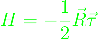
Then, the first two energy-eigenvalues obtained through Zeeman splitting can be obtained as ± 1/2 R. The R-dependent ground-state written as

This parametrization will of course have a discontinuity at one of the poles (the one that's not the zero-coordinate). This is just a topological reality, called the "hairy-ball theorem" or "hedgehog theorem". It's up to the observer to pick a appropriate parametrization.
The Berry-phase can be alternatively written as an integral over the Berry curvature, which is finally gauge invariant. It's divergence-free and always has a representation as a curl on contractible parameter manifolds as per Poincare's lemma.

which means that depending on the Hamiltonian, the Berry-curvature looks like the field of a magnetic monopole. It's singularly where the magnetic charge sits. The corresponding vector potential models a Dirac string to extend towards the other side of the usual dipole. It of course doesn't do anything apart from accommodating the field theory by shifting the singularity away from the point where a magnetic dipole would create it.

The Berry phase then is the flux of the magnetic field through a surface bounded by C. This effectively builds two complementary hemispheres. Define the Chern number

This concept may be generalized to arbitrary real axes. In the toy model, the manifold M exists in 3 real dimensions, discounting {0}. For contractible M, then C = 0 globally. As such, the Chern number depends heavily on the integration curve. The non-trivial topology (i.e. C ≠ 0) requires non-trivial parameter manifolds. In the toy model, and S the surface of a R-ball, then C = -1. Inductively,

Begin with the tight-binding Hamiltonian of independent fermions on a lattice

where {t(k)} is a bundle of 2x2 Bloch Hamiltonians on S. All these t(k) derive from H. This can be expanded into a basis of Hermitian 2x2 matrices.

In the Qi-Wu-Zhang model, t(k) is parametrized so that ε describes two bands with periodic structure. To get the Chern number, treat t(k) as H(R) in the toy model, so

The physical parameter manifold is the 1BZ, so the map d is smooth. The image of the 1BZ under d is 2-dimensional, closed and can define infinitesimal surface element. This means that the Hamiltonian may be continuously deformed. The Chern number remains constant though (unless a gap closure occurs).
Bosonic Ensembles
At second quantization, quantum mechanics emerge in which states and observables can be written in terms of particle operators exclusively. These should be expressible using an ONB of common eigenstates of these operators. The question is, whether this representation of quantum mechanics is workable. Define coherent states |y⟩

Using these states will represent operators as diagonal matrices with easily computable diagonal elements. The existence of these coherent states is not immediately obvious.
The Fock-space spanned by an ONB will treat coherent states essentially as an eigenvalue problem for the particle operators. Under the assumption that coherent states can be normalized, then there is some finite integer N₀ with a state that evaluates to zero for all smaller N, and

This means that at some N₀, the creation operator doesn't actually lift the state, which is of course definitionally problematic. This means that coherent states can't be normalized, and it's not a common eigenstate of all creation operators. The converse however is true, although the eigenvalue is not generally real, but complex. The annihilator then is not generally hermitian.

From that we can infer that coherent states don't form an ONB, since they're neither normalized, nor orthogonal. It still needs to be a basis, so we infer that it's overcomplete.

The holomorphic representation of a state in the Fock-space using coherent space is

The exponential function is holomorphic on the y*, hence why this is called the "holomorphic representation". It's convenient, since it's definition is an analogue to the position representation. This is also the basis in which the particle operators are associated with the derivatives:

The partition function using the number state ONB is written as

A Quantum Mechanical Description of Magnetism and Numerical Methods
Magnetism is a relatively heterogeneous phenomenon. Magnetic moments can be itenerant (traveling through the structure) or localized, there is trivially the (anti-)ferromagnetic distinction, and each type of metal and insulator comes with a model that best describes its physics. Generally, all materials are paramagnetic at high temperatures. Ferromagnetic materials become so below their Curie temperature, and anti-ferromagnetic materials below their Neel temperature. They are described by the Stoner theory and Slater model respectively. Both can be derived from the Hubbard model's Mean-Field theory.
For classification purposes, metallic, itinerant ferromagnetism carries no localized spin, but instead gets strong Coulomb interaction. The electrons are assumed to be non-degenerate and living in narrow 3-dimensional bands. A high density of states at the Fermi energy of course favours ferromagnetism through the minimized interaction energy, and only slight increase of kinetic energy This can be written as the "Stoner criterium"

The Hartree-Fock approximation of the Hubbard-model is found mostly through rewriting the occupation number operators to find the fluctuation terms to ignore.

Since the magnetic structures are periodic, the solution should be translationally invariant.

For a better description of the electron-density and magnetization, it's better to switch to the momentum space and perform a Fourier back-transformation.

This makes the paramagnetic solution the trivial one, and where m > 0 solutions exist, the mirrored version is also possible. For a temperature tending to infinity, β goes to 0. Similarly for the case m = 0, the temperature tends to infinity. Approaching the Curie temperature from below will result in small magnetization with the first non-trivial order in the expansion yielding the conditional equation for the Curie temperature:

By checking the behavior of a Curie-temperature tending to zero, one can recover the Stoner criterion

The ferromagnetic order of local spins minimizes the interaction energy, so there will only be interactions between electrons of complementary spin. This is in agreement with the Pauli principle, since it acts as effective repulsion for particles with parallel spin. Acting against that with enhanced kinetic energy assumes the parallel spin electron having previously occupied higher states of energy. This means that strong interaction energy and a high density of states at Fermi-energy are favourable for ferromagnetism. The Curie temperature is about the same as the interaction energy for systems, where the interaction energy is strong. This implies that anti-ferromagnetic order is realized at half-filling. The high interaction energy being about the same as the Curie temperature is a bit questionable, which has unfortunate implications for mean-field theory. The solution to that is to introduce a critical exponent for the magnetization, which we get for checking the magnetization at the Curie temperature.

This coincides with the classical Landau result for the critical exponent.
The idea of "solving" the Hubbard model completely is a little naive, and can only be tackled numerically due to their man degrees of freedom. It's a question of solving a Hamiltonian, which in these dimensions is best done using linear algebra. This begins with the linear diagonalization to reveal the eigenvalues (i.e. energy-eigenstates). It's probably easiest to look for the smallest eigenvalue so the other eigenstates can be inferred pretty directly. To expedite the process, one can try to identify symmetries to exploit. One of these is the conservation of total particle number, which can be extended to each spin-projection (i.e. particle conservation + spin conservation). The Power Method sees an initial state with the relation

The gap between energy eigenstates will determine the rate of convergence. This method is handy, because it only requires two vectors to be stored at a time, but it's surpassed by the Lanczos Approach. A random initial vector can be expanded into a sum of vectors from an ONB. Write the Hubbard model as a matrix again. The n-th Krylov space of this vector then is

Then, iteratively

The vectors v then build an ONB of Krylov space.
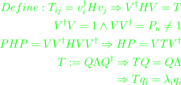
Which defines {q} as the Lanczos basis. The orthonormal eigenvectors of H correspond to the eigenvalues of Λ. The time-evolution for Krylov Approaach introduces the matrix product PHP as the exact action of the Hamiltonian. As such,
